ROI Navigator — user guide
ROI Navigator is a tool for analysing and modelling future business performance based on predictive sales models. It shows which factors drive sales and how much each of them contributes: price, distribution, promo, assortment, seasonality, competitor activity and media support. With ROI Navigator you can compare a brand with its competitors, forecast sales for different scenarios, estimate sales elasticity to price and distribution, find the right media mix for a given budget and check model quality. This guide covers the Analysis, Sales scenarios, Elasticities and Technical charts sections.
Analysis
This section lets you view and analyse the results of sales modelling over the historical period.
To get started, choose a category, a brand and competitors from the drop-down lists at the top of the Analysis tab. Depending on the source data used for modelling, subcategory and geography selection may also be available.
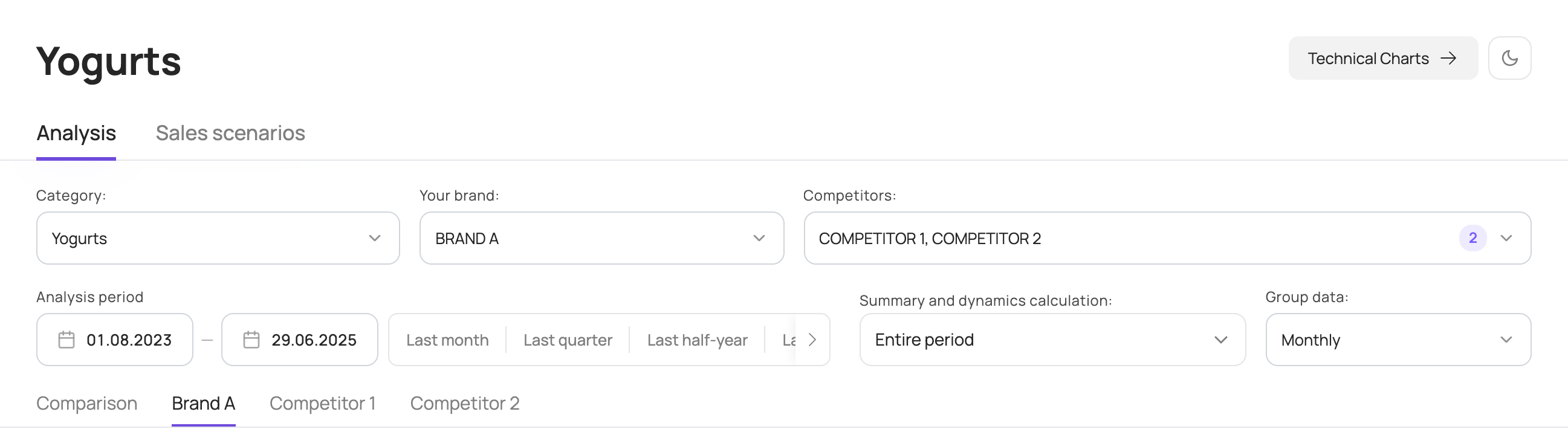
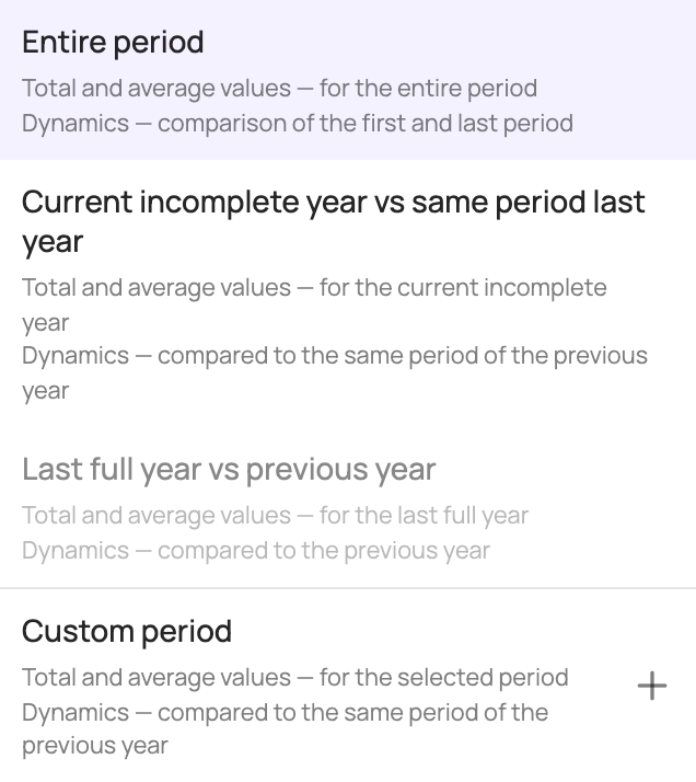
By default, the entire analysis period is selected, starting from the 1st day of the first full month of the analysed period. You can change the period shown on the charts by picking dates in the calendar. You can also change the comparison period used to calculate the summary figures and dynamics above the charts. The following calculation options are available:
| Option | What it shows |
|---|---|
| “Entire period” | Total and average values for the entire period; dynamics compare the first and the last period. Selected by default. |
| “Current incomplete year vs same period last year” | Total and average values for the current incomplete year; dynamics compare it with the same period last year. |
| “Last full year vs previous year” | Total and average values for the last full year; dynamics compare it with the previous year. Available when the analysis period includes 2 full calendar years. |
| “Custom period” | Total and average values for the selected period; dynamics compare it with the same period last year. |
You can also change how data is grouped by period. By default, chart data is grouped by month; you can switch to weeks, quarters, half-years or years.
Analytical charts can be viewed either separately for the selected brand and competitors or as a comparison of the selected brands. To do this, open a brand tab or the Comparison tab.
Brand tab
If the source data for modelling was split by SKU, you can choose subcategories or specific SKUs on the left of the screen to show on the charts.
The following charts are available for the selected brand and competitors:
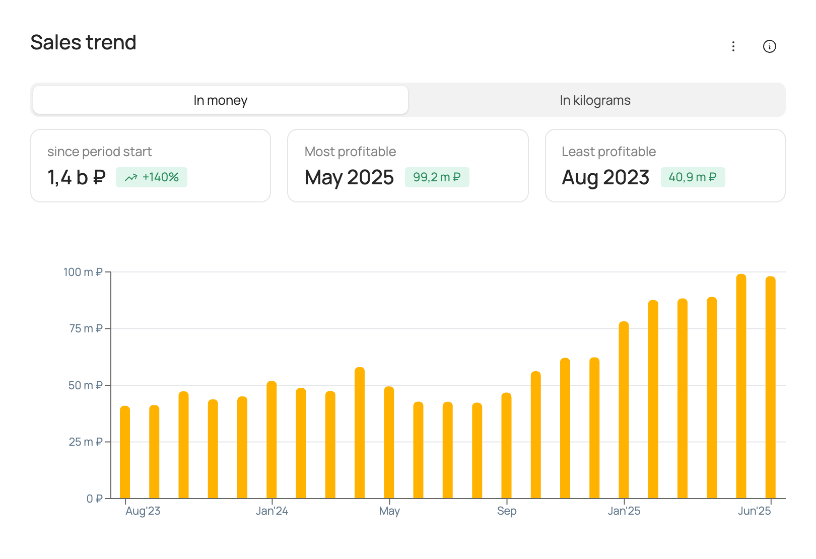
Sales trend
The chart shows actual sales in roubles and volume over the analysis period at the selected frequency (weekly/monthly/quarterly/half-yearly/yearly) for the selected brand.
| Box | What it shows |
|---|---|
| “since period start” | The brand's total sales in roubles/volume, depending on the option selected on the chart, and the change in these sales over the analysis period. |
| “Most profitable” | The period with the brand's highest sales in roubles/volume, depending on the option selected on the chart, and the sales for that period. |
| “Least profitable” | The period with the brand's lowest sales in roubles/volume, depending on the option selected on the chart, and the sales for that period. |
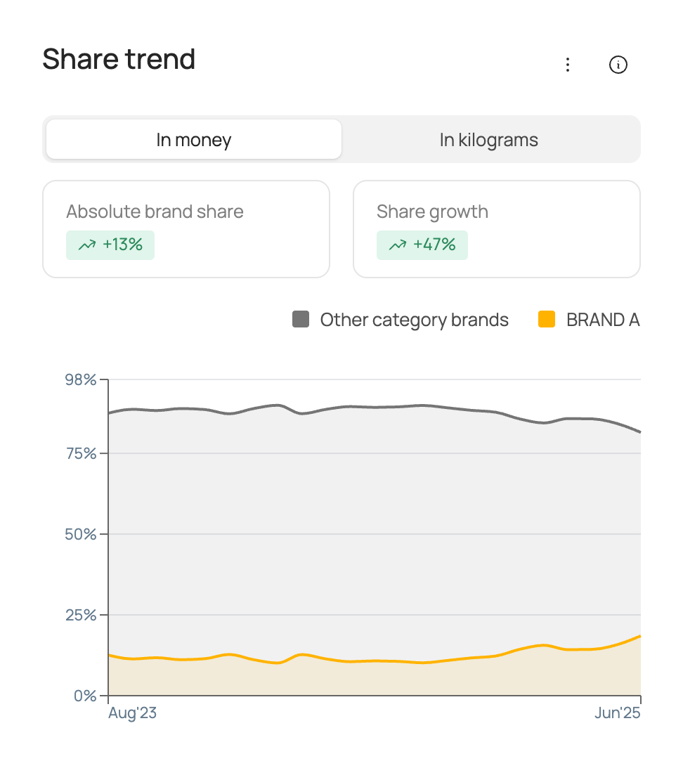
Share trend
The chart shows the market share of total category sales over the analysis period at the selected frequency (weekly/monthly/quarterly/half-yearly/yearly) for the selected brand and for the other brands in the category combined.
| Box | What it shows |
|---|---|
| “Absolute brand share” | The selected brand's market share for the comparison period. Market share is calculated in roubles/volume, depending on the option selected on the chart, from total category sales. |
| “Share growth” | The growth of the selected brand's market share for the comparison period. Market share is calculated in roubles/volume, depending on the option selected on the chart, from total category sales. |
Factor contribution to sales
The chart shows the contribution of each factor to the selected brand's sales over the analysis period. Contributions are shown in roubles/volume, depending on the option selected on the chart.
| Box | What it shows |
|---|---|
| “Top by absolute contribution” | The factor with the largest contribution to brand sales in roubles/volume, depending on the option selected on the chart, and the value of its contribution for the comparison period. |
| “Top by contribution growth” | The factor with the largest growth / smallest decline in contribution to brand sales in roubles/volume, depending on the option selected on the chart, and the change in its contribution for the comparison period. |
| “Lowest contribution” | The factor with the smallest contribution to brand sales in roubles/volume, depending on the option selected on the chart, and the value of its contribution for the comparison period. |
| “Total price contribution” | The contribution of price factors to brand sales in roubles/volume, depending on the option selected on the chart, for the comparison period. |
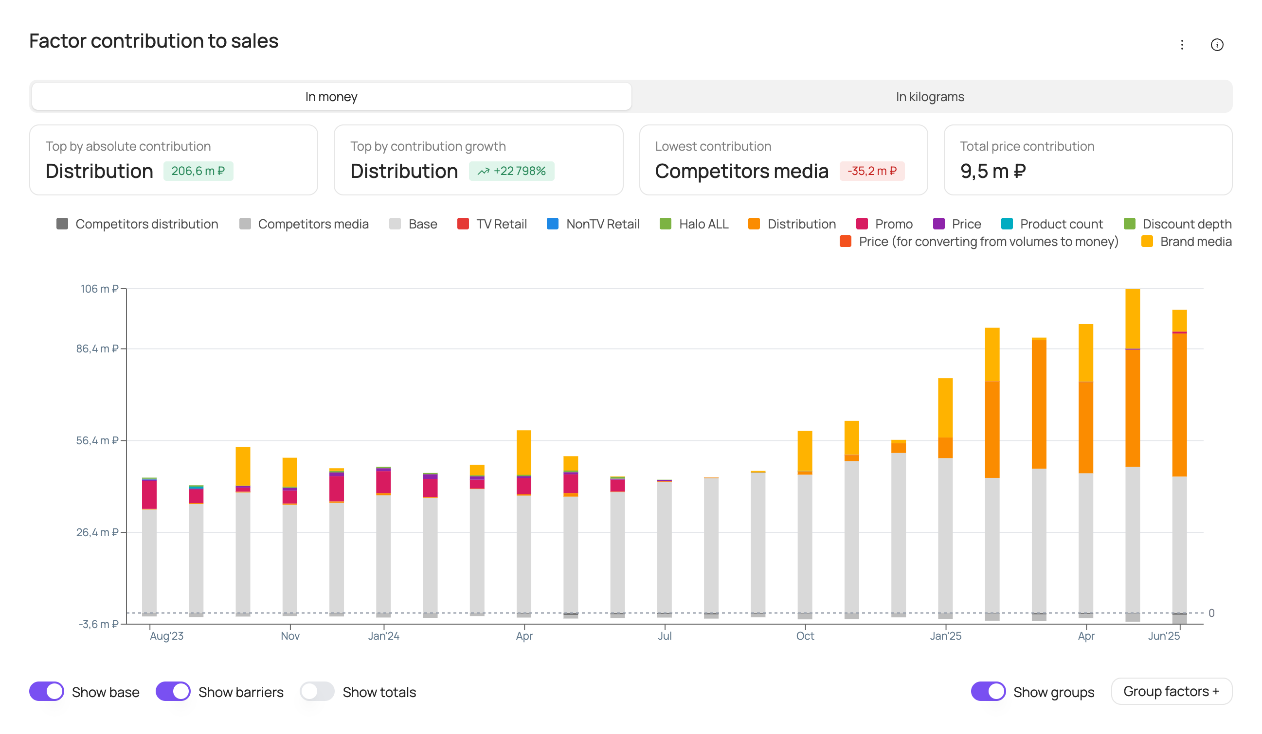
At the bottom of the chart you can turn the following elements on or off: base (the brand's base sales), barriers (negative factors), totals (sales labels above each bar).
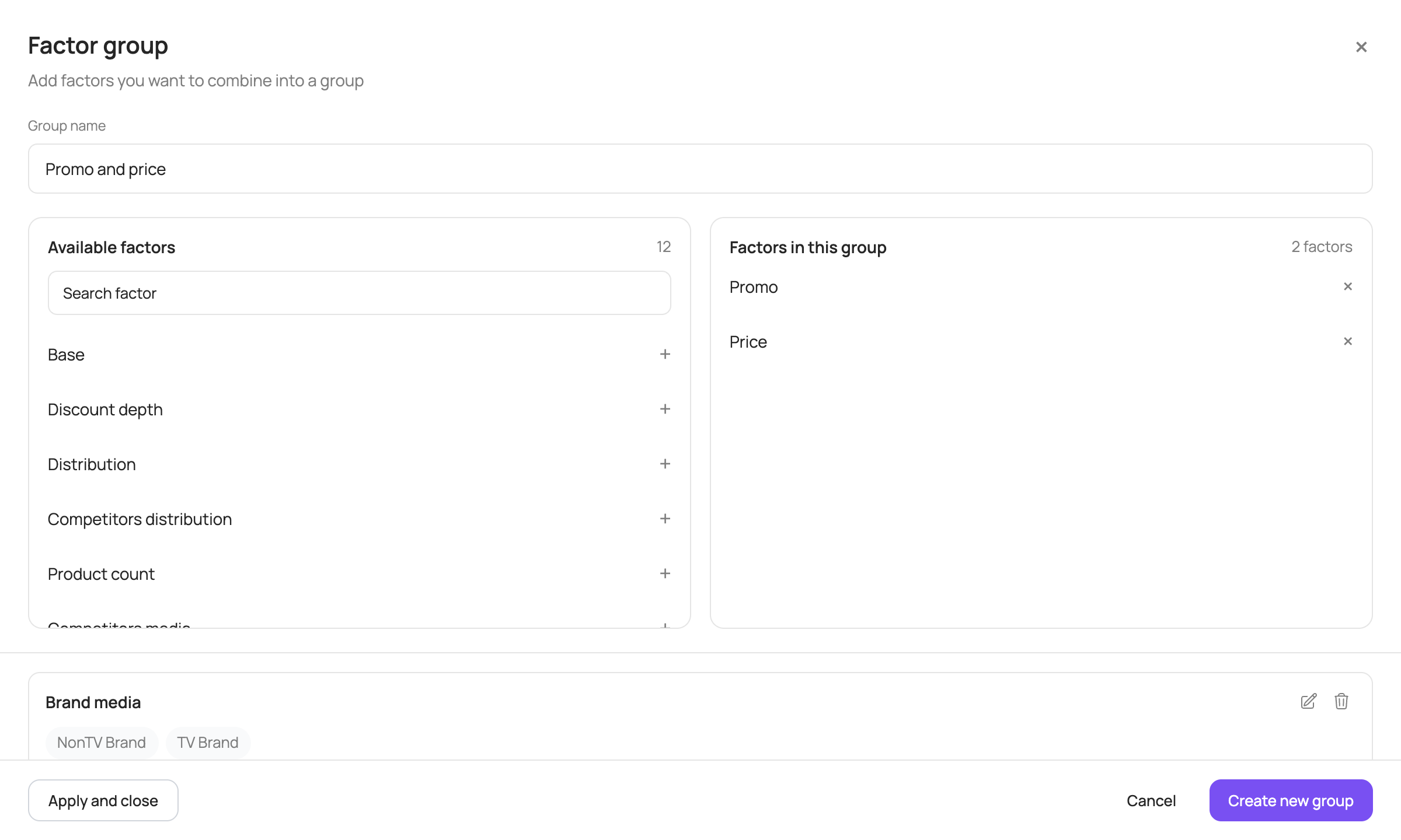
In addition, the “Group factors +” button is available at the bottom right of the chart. It lets you combine several factors into a group and show their total contribution as a single bar: in the “Factor group” window, enter a group name, add at least 2 factors and click “Create new group”, then “Apply and close”. Groups you create can be edited or deleted. The “Show groups” toggle temporarily brings back individual factors on the chart.
Price trend
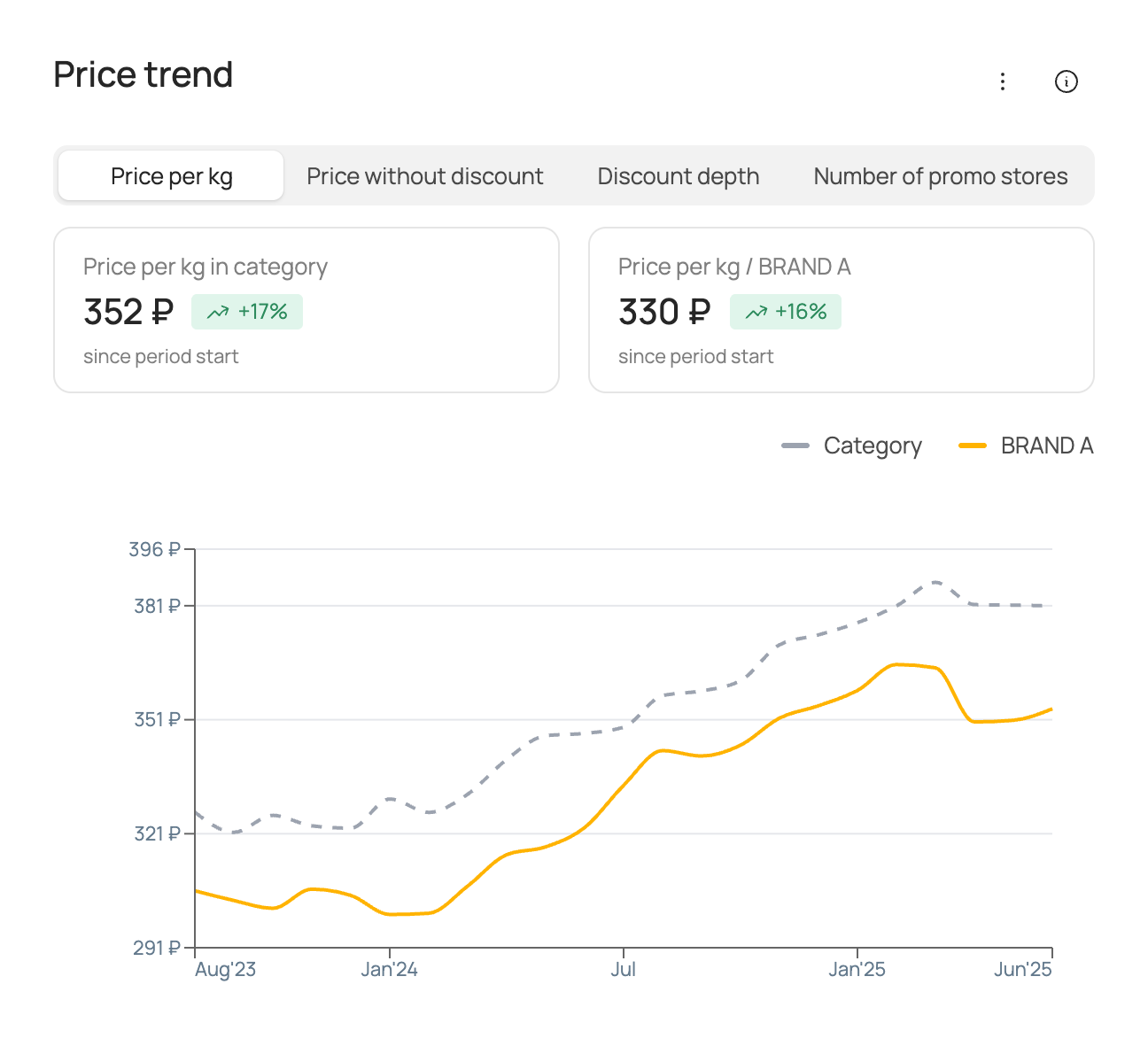
The chart shows the actual values of the price factor over the analysis period at the selected frequency (weekly/monthly/quarterly/half-yearly/yearly) for the selected brand and for the category as a whole. The set of price factors may vary depending on the source data used for modelling.
Box names follow the price factor selected above the chart.
| Box | What it shows |
|---|---|
| “… in category” | The average value of the price factor in the category and its change over the comparison period. |
| “… / brand” | The average value of the brand's price factor and its change over the comparison period. |
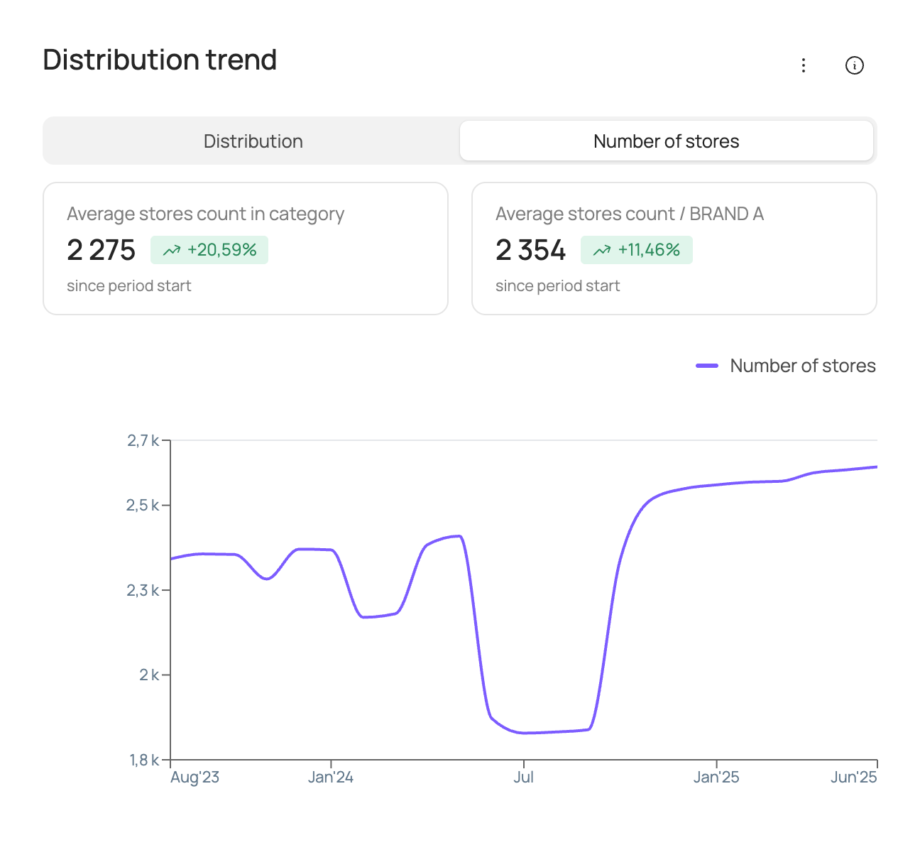
Distribution trend
The chart shows the actual values of the distribution factor over the analysis period at the selected frequency (weekly/monthly/quarterly/half-yearly/yearly) for the selected brand and for the category as a whole. The set of distribution factors may vary depending on the source data used for modelling.
For the “Number of stores” factor, the boxes are called “Average stores count in category” and “Average stores count / brand”.
| Box | What it shows |
|---|---|
| “Average weighted distribution in category” | The average value of the distribution factor in the category and its change over the comparison period. |
| “Average weighted distribution / brand” | The average value of the brand's distribution factor and its change over the comparison period. |
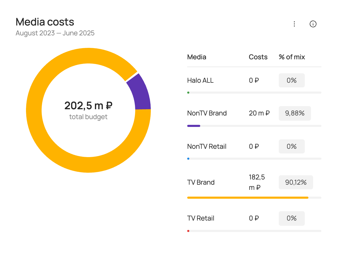
Media costs
Shows advertising spend for the selected analysis period.
Media support is split into the following groups:
| Group | Description |
|---|---|
| TV Brand | Image advertising of the brand on TV. |
| TV Retail | Co-promo advertising of the brand with retailers on TV. |
| NonTV Brand | Image advertising of the brand in other media channels (radio, OOH, digital). |
| NonTV Retail | Co-promo advertising of the brand with retailers in other media channels (radio, OOH, digital). |
| Halo ALL | Advertising of the brand's other products. |
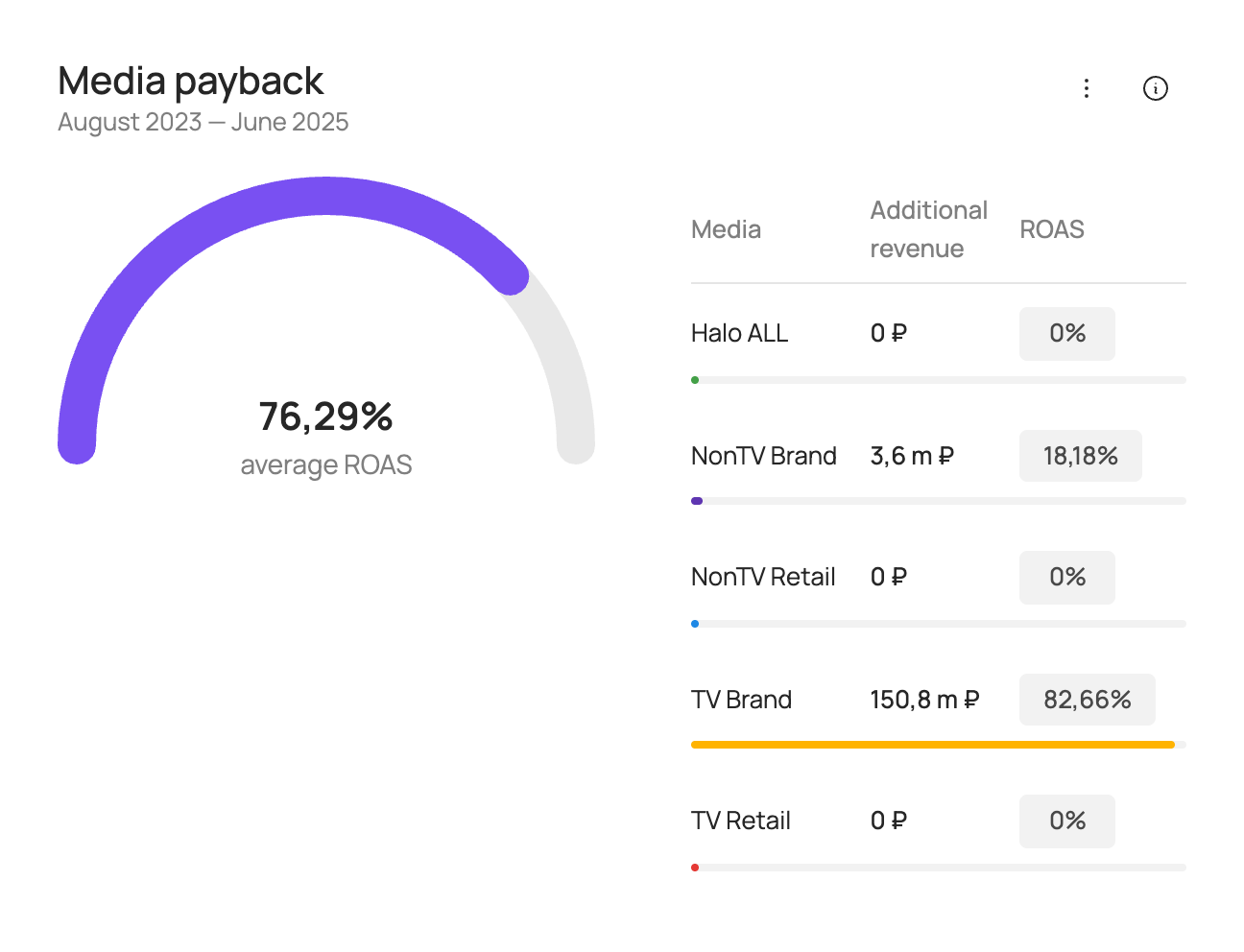
Media payback
Shows additional revenue in roubles from advertising and ROAS for the selected analysis period.
ROAS (return on ad spend) is a measure of media investment efficiency. ROAS > 100% means that advertising investment pays off through additional sales revenue.
ROAS is calculated as:
Media support is split into the following groups:
| Group | Description |
|---|---|
| TV Brand | Image advertising of the brand on TV. |
| TV Retail | Co-promo advertising of the brand with retailers on TV. |
| NonTV Brand | Image advertising of the brand in other media channels (radio, OOH, digital). |
| NonTV Retail | Co-promo advertising of the brand with retailers in other media channels (radio, OOH, digital). |
| Halo ALL | Advertising of the brand's other products. |
Comparison tab
If the source data for modelling was split by SKU, you can choose a brand comparison or build your own comparison of 2–10 SKUs on the left of the screen to show on the charts.
The following charts are available for the selected brand and competitors:
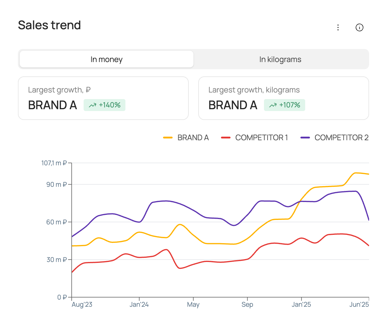
Sales trend
The chart shows actual sales over the analysis period at the selected frequency (weekly/monthly/quarterly/half-yearly/yearly) for the selected brand and competitors.
| Box | What it shows |
|---|---|
| “Largest growth, ₽” | The brand with the largest sales growth in roubles and its sales growth in percent for the comparison period among the selected brands. |
| “Largest growth, kilograms” | The brand with the largest sales growth in volume and its sales growth in percent for the comparison period among the selected brands. |
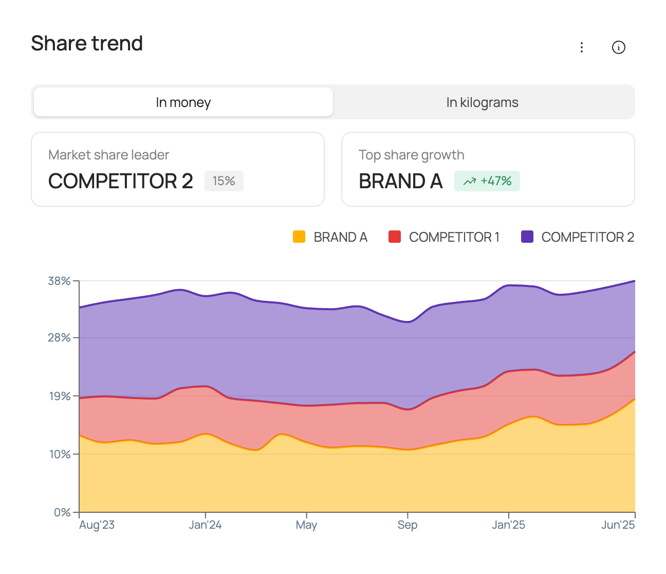
Share trend
The chart shows the market share of total category sales over the analysis period at the selected frequency (weekly/monthly/quarterly/half-yearly/yearly) for the selected brand and competitors.
| Box | What it shows |
|---|---|
| “Market share leader” | The brand leading by market share for the comparison period and that brand's market share. Market share is calculated in roubles/volume, depending on the option selected on the chart, from total category sales. |
| “Top share growth” | The brand leading by share growth for the comparison period. Market share is calculated in roubles/volume, depending on the option selected on the chart, from total category sales. |
Factor contribution to sales
The chart shows the contribution of each factor to the sales of the selected brand and competitors over the analysis period. Contributions are shown in roubles/volume, depending on the option selected on the chart.
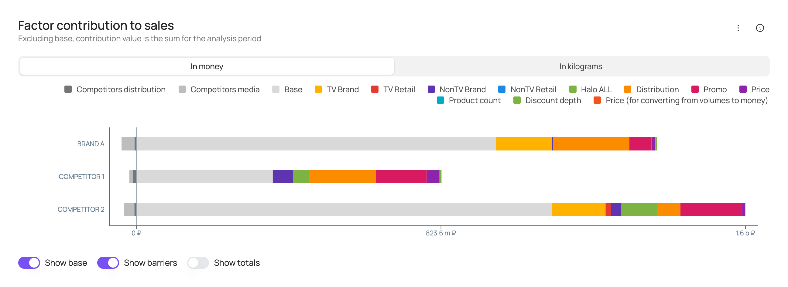
At the bottom of the chart you can turn the following elements on or off: base (the brand's base sales), barriers (negative factors), totals (sales labels above each bar).
Price trend
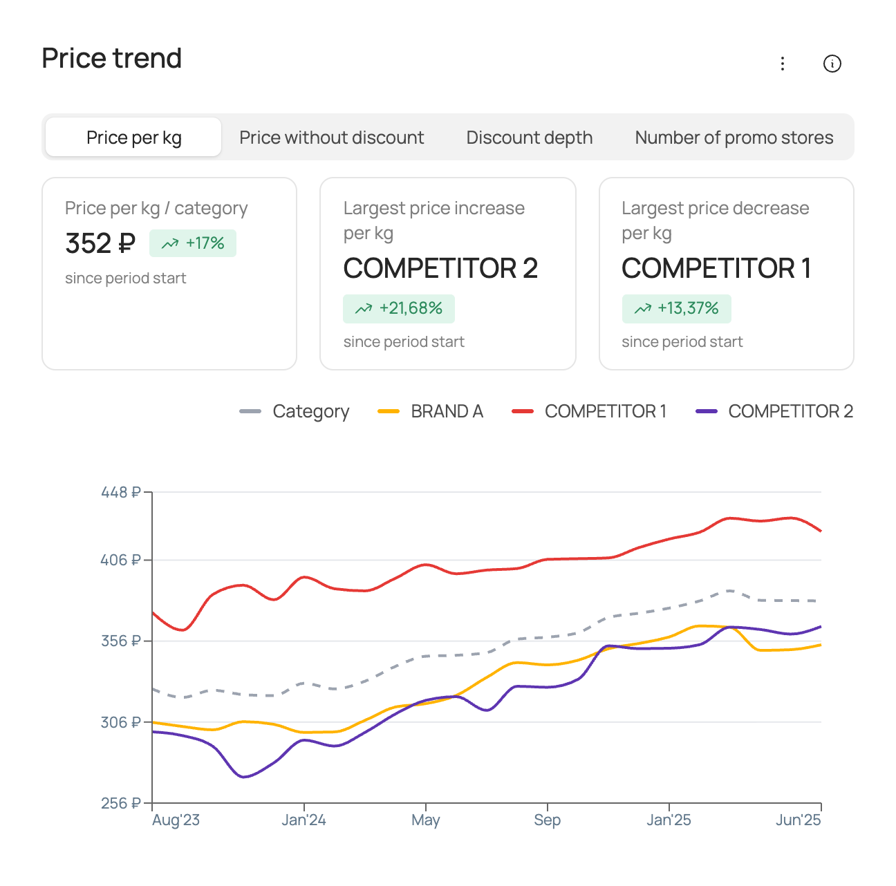
The chart shows the actual values of the price factor over the analysis period at the selected frequency (weekly/monthly/quarterly/half-yearly/yearly) for the selected brand, competitors and the category as a whole. The set of price factors may vary depending on the source data used for modelling.
| Box | What it shows |
|---|---|
| “… / category” | The average value of the price factor in the category and its change over the comparison period. |
| “Largest price increase” | The brand with the largest increase / smallest decrease of the price factor for the comparison period and the change of the price factor for that brand. |
| “Largest price decrease” | The brand with the largest decrease / smallest increase of the price factor for the comparison period and the change of the price factor for that brand. |
Distribution trend
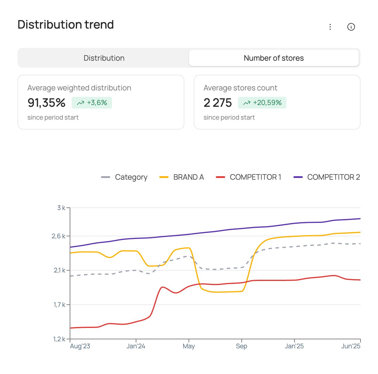
The chart shows the actual values of the distribution factor over the analysis period at the selected frequency (weekly/monthly/quarterly/half-yearly/yearly) for the selected brand, competitors and the category as a whole. The set of distribution factors may vary depending on the source data used for modelling.
| Box | What it shows |
|---|---|
| “Average weighted distribution” | The average weighted distribution in the category and its change over the comparison period. |
| “Average stores count” | The average number of stores in the category and its change over the comparison period. |
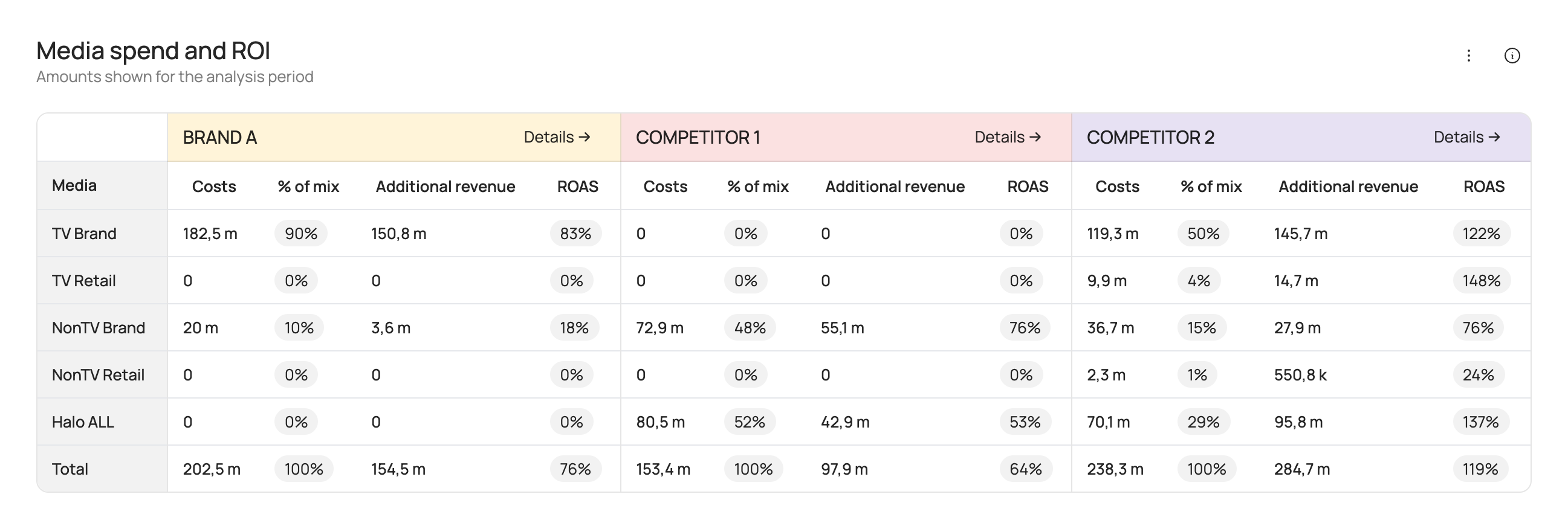
Media spend and ROI
The table shows advertising spend, additional revenue in roubles from advertising and ROAS for the selected analysis period.
ROAS (return on ad spend) is a measure of media investment efficiency. ROAS > 100% means that advertising investment pays off through additional sales revenue.
ROAS is calculated as:
Media support is split into the following groups:
| Group | Description |
|---|---|
| TV Brand | Image advertising of the brand on TV. |
| TV Retail | Co-promo advertising of the brand with retailers on TV. |
| NonTV Brand | Image advertising of the brand in other media channels (radio, OOH, digital). |
| NonTV Retail | Co-promo advertising of the brand with retailers in other media channels (radio, OOH, digital). |
| Halo ALL | Advertising of the brand's other products. |
Sales scenarios
This section lets you forecast future sales for different media support scenarios and other factors.
At the top of the tab you can change the category and brand. Depending on the source data used for modelling, subcategory and geography selection may also be available. You can also change the forecast period. The minimum period is 1 month, the maximum period is 1 year.
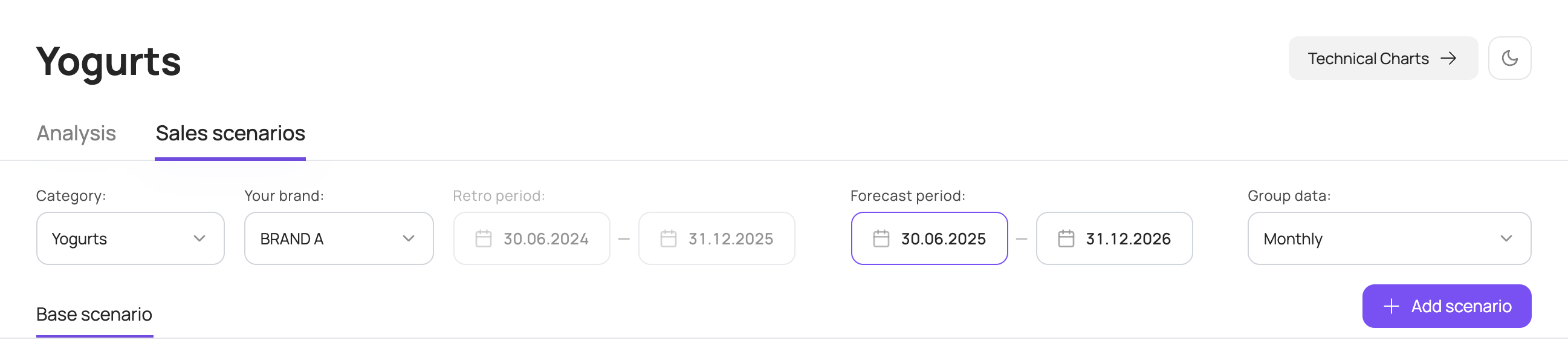
You can also change how data is grouped by period. By default, chart data is grouped by month; you can switch to weeks, quarters, half-years or years.
If the source data for modelling was split by SKU, you can choose subcategories or specific SKUs on the left of the screen to show on the charts.
Base scenario
By default, the base scenario for the selected forecast period is shown. It includes actual data for the period already included in the model and forecast data for the rest of the period.
The base scenario uses the following forecast data:
- media activity is set to the same placement volumes as in the same period last year;
- seasonality corresponds to each specific week;
- the category sales factor is forecast by trend;
- other factors use average values over the last 8 available weeks included in the model.
The scenario overview in the top left shows the key figures for the forecast period: sales forecast in roubles and volume, average price, total media investment and ROAS for the selected forecast period.
ROAS (return on ad spend) is a measure of media investment efficiency. ROAS > 100% means that advertising investment pays off through additional sales revenue.
ROAS is calculated as:
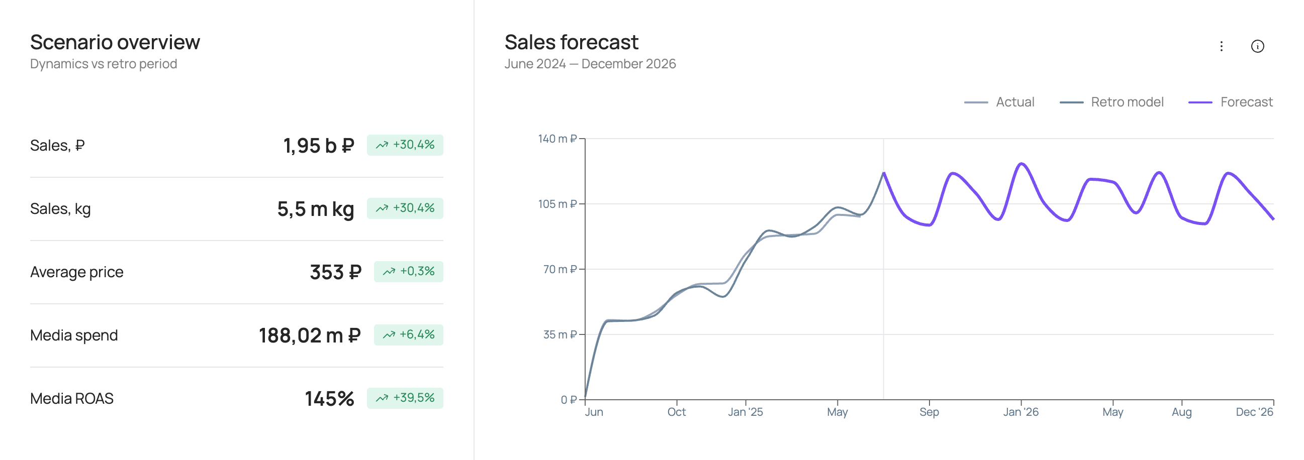
The following charts are also available in the scenario:
Sales forecast
The chart shows the brand's sales forecast in roubles for the selected forecast period and for the retro period at the selected frequency (weekly/monthly/quarterly/half-yearly/yearly).
Factor contribution forecast
The chart shows the contribution of each factor to brand sales over the selected forecast period at the selected frequency (weekly/monthly/quarterly/half-yearly/yearly).
| Box | What it shows |
|---|---|
| “Top by absolute contribution (excluding base)” | The factor with the largest contribution to brand sales in roubles and the value of its contribution over the selected forecast period. |
| “Top by contribution growth (excluding base)” | The factor with the largest growth / smallest decline in contribution to brand sales in roubles and the change in its contribution over the selected forecast period relative to the retro period. |
| “Price contribution” | The contribution of price factors to brand sales in roubles over the selected forecast period. |
| “Least profitable” | The period with the lowest sales in roubles within the selected forecast period. |
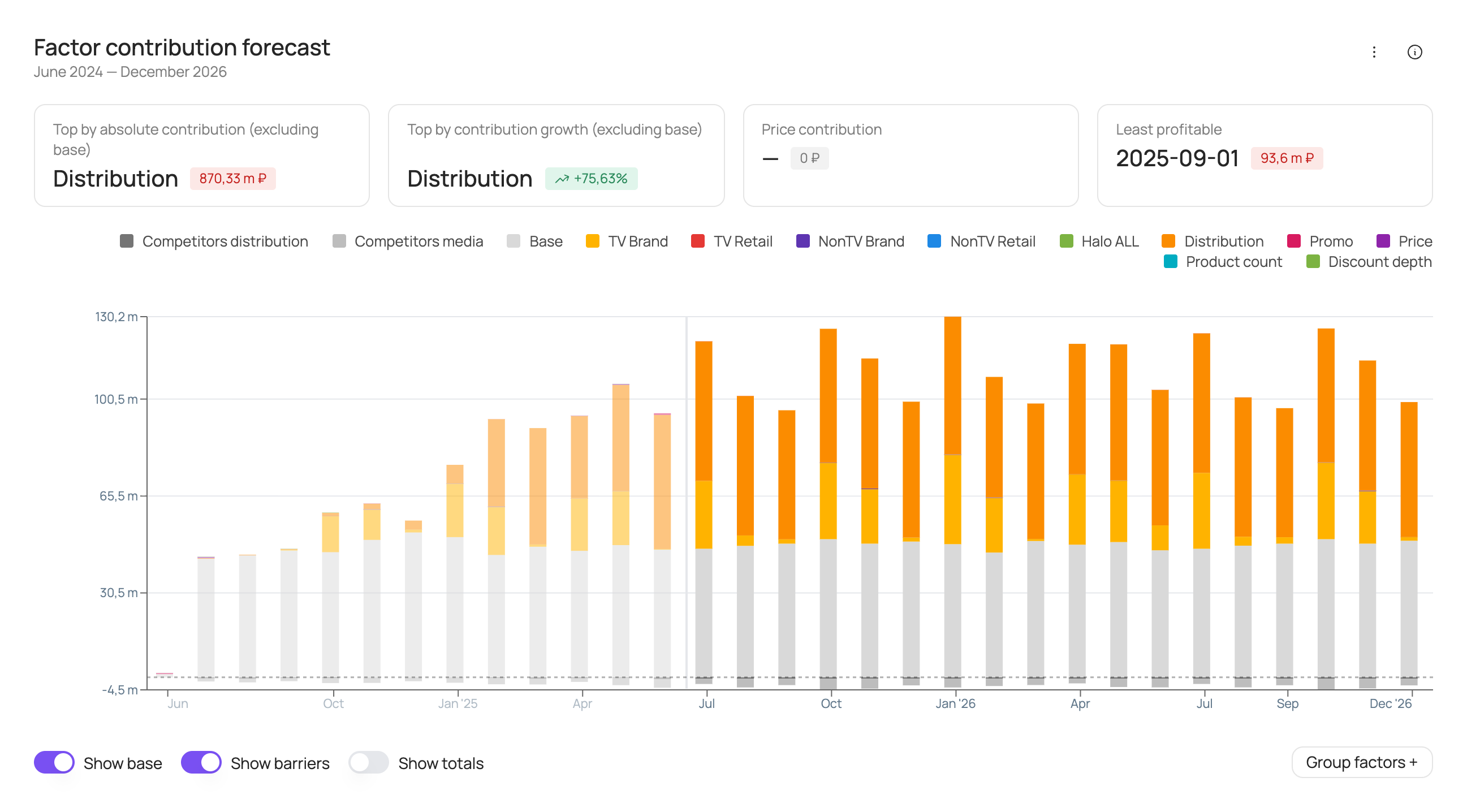
At the bottom of the chart you can turn the following elements on or off: base (the brand's base sales), barriers (negative factors), totals (sales labels above each bar).
In addition, the “Group factors +” button is available at the bottom right of the chart. It lets you combine several factors into a group and show their total contribution as a single bar: in the “Factor group” window, enter a group name, add at least 2 factors and click “Create new group”, then “Apply and close”. Groups you create can be edited or deleted. The “Show groups” toggle temporarily brings back individual factors on the chart.
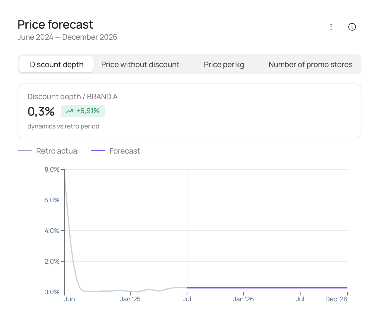
Price forecast
The chart shows the values of price factors for the forecast period and the retro period at the selected frequency (weekly/monthly/quarterly/half-yearly/yearly).
The box name follows the price factor selected above the chart, for example “Discount depth / brand”.
| Box | What it shows |
|---|---|
| “… / brand” | The average value of the price factor and its change over the selected forecast period relative to the retro period. |
Distribution forecast
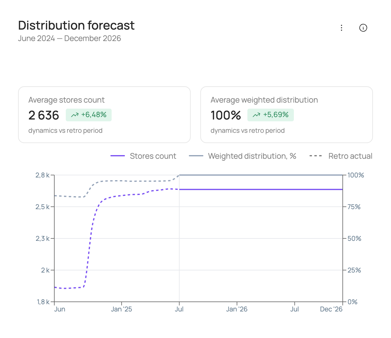
The chart shows the values of distribution factors for the forecast period and the retro period at the selected frequency (weekly/monthly/quarterly/half-yearly/yearly).
| Box | What it shows |
|---|---|
| “Average stores count” | The average value of the distribution factor and its change over the selected forecast period relative to the retro period. |
| “Average weighted distribution” | The average value of the distribution factor and its change over the selected forecast period relative to the retro period. |
Media costs
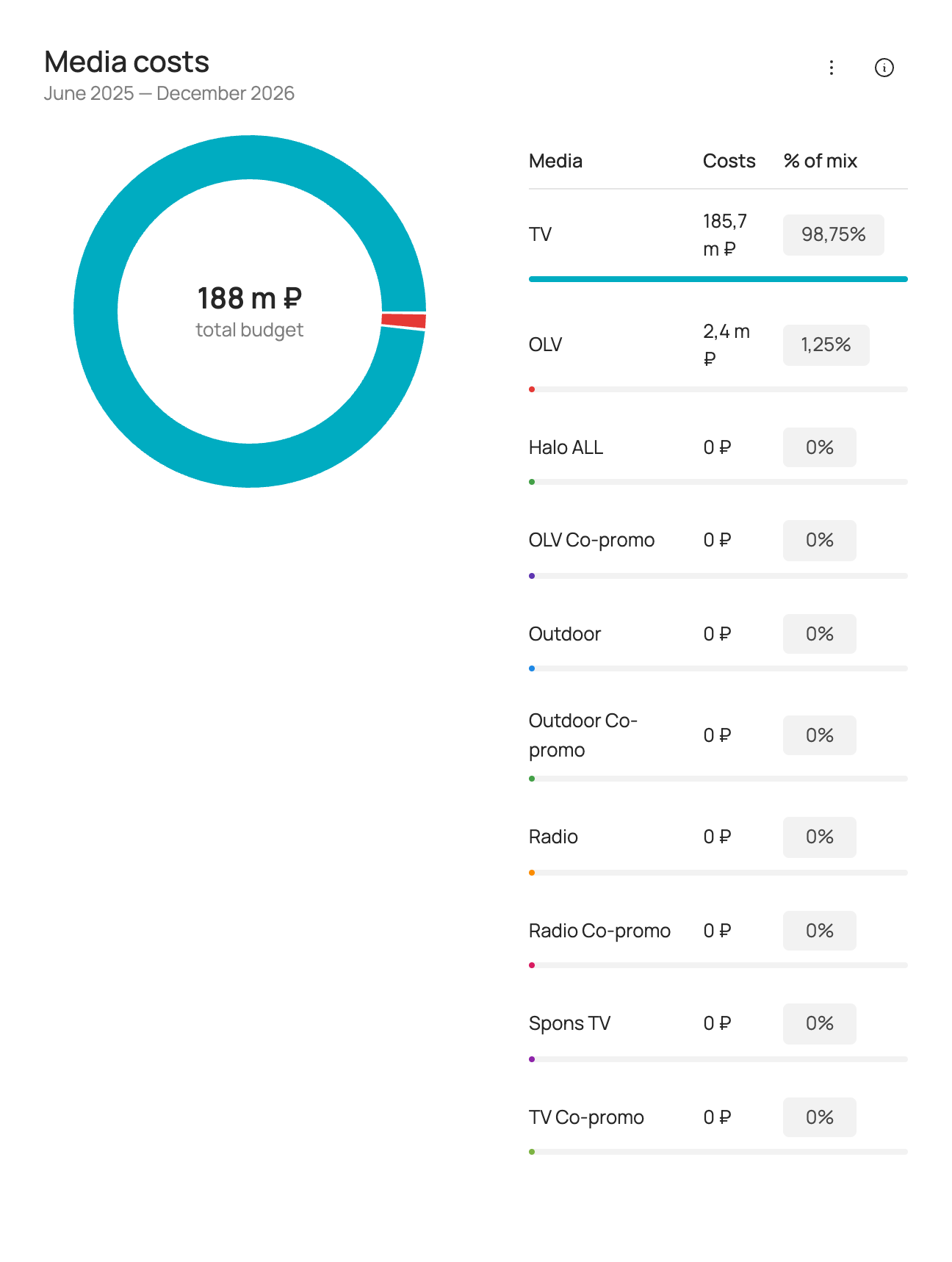
Shows advertising spend for the selected forecast period.
Media support is split into the following groups:
| Group | Description |
|---|---|
| TV | Image advertising of the brand on TV. |
| TV Co-promo | Co-promo advertising of the brand with retailers on TV. |
| OLV | Image advertising of the brand in online video. |
| OLV Co-promo | Co-promo advertising of the brand with retailers in online video. |
| Outdoor | Image outdoor advertising of the brand. |
| Outdoor Co-promo | Outdoor co-promo advertising of the brand with retailers. |
| Radio | Image advertising of the brand on radio. |
| Radio Co-promo | Co-promo advertising of the brand with retailers on radio. |
| Halo ALL | Advertising of the brand's other products. |
Media payback
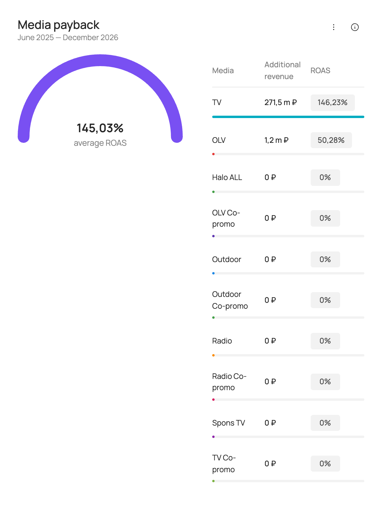
Shows additional revenue in roubles from advertising and ROAS for the selected forecast period.
ROAS (return on ad spend) is a measure of media investment efficiency. ROAS > 100% means that advertising investment pays off through additional sales revenue.
ROAS is calculated as:
Media support is split into the following groups:
| Group | Description |
|---|---|
| TV | Image advertising of the brand on TV. |
| TV Co-promo | Co-promo advertising of the brand with retailers on TV. |
| OLV | Image advertising of the brand in online video. |
| OLV Co-promo | Co-promo advertising of the brand with retailers in online video. |
| Outdoor | Image outdoor advertising of the brand. |
| Outdoor Co-promo | Outdoor co-promo advertising of the brand with retailers. |
| Radio | Image advertising of the brand on radio. |
| Radio Co-promo | Co-promo advertising of the brand with retailers on radio. |
| Halo ALL | Advertising of the brand's other products. |
Creating a new scenario — manually
- In the top right corner of the Sales scenarios tab, click “Add scenario”. A new scenario can be created in two ways: manually (via the interface) or using a template (by uploading an Excel file).
- To create a scenario manually, enter the scenario name, choose the calculation type for media parameters and the input type for factor values.
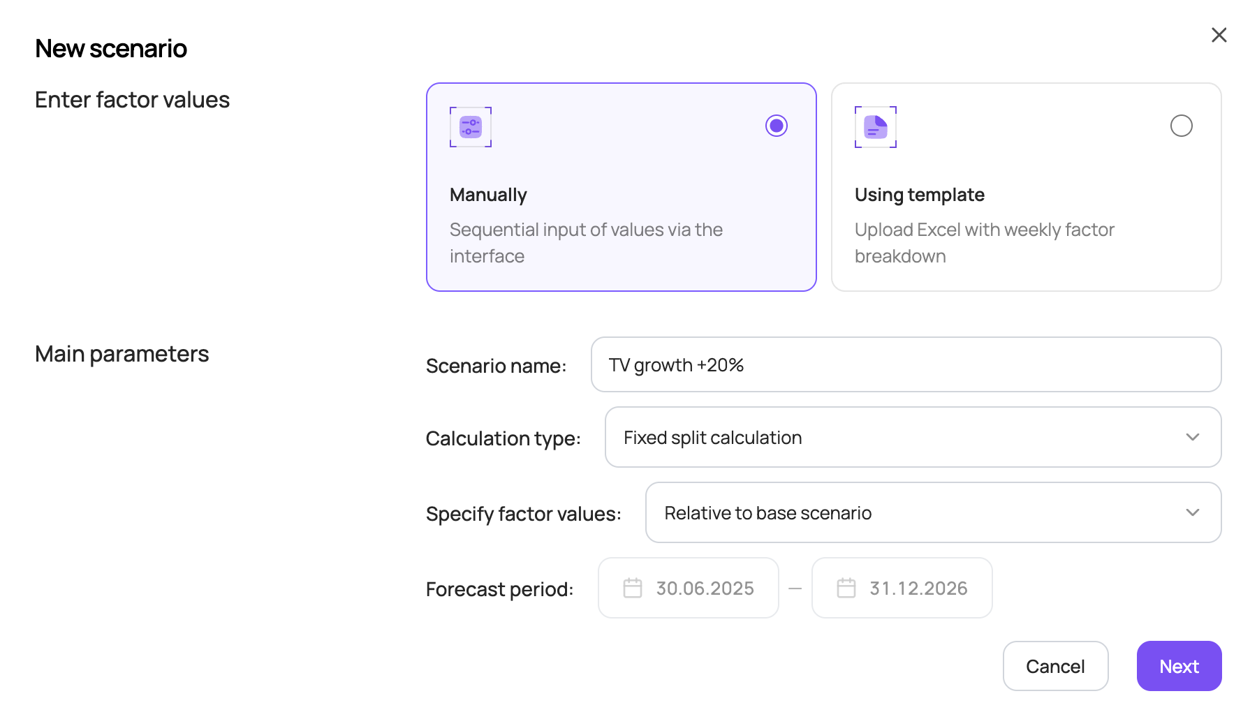
Two calculation options are available for media parameters:
- “Fixed split calculation” — a table with cost and budget is filled in for each media channel;
- “Maximize sales within a given budget” — the tool automatically selects the optimal media mix for the given budget, taking into account the constraints entered for each media channel.
Two options are available for entering the values of other factors:
- “Relative to base scenario” — use sliders to increase/decrease factor values relative to the base scenario;
- “Exact value” — enter specific values for each factor. This option is not available for granular models by region/SKU.
The forecast period is shown for reference. To change it, go back to the Sales scenarios page.
Non-media factors
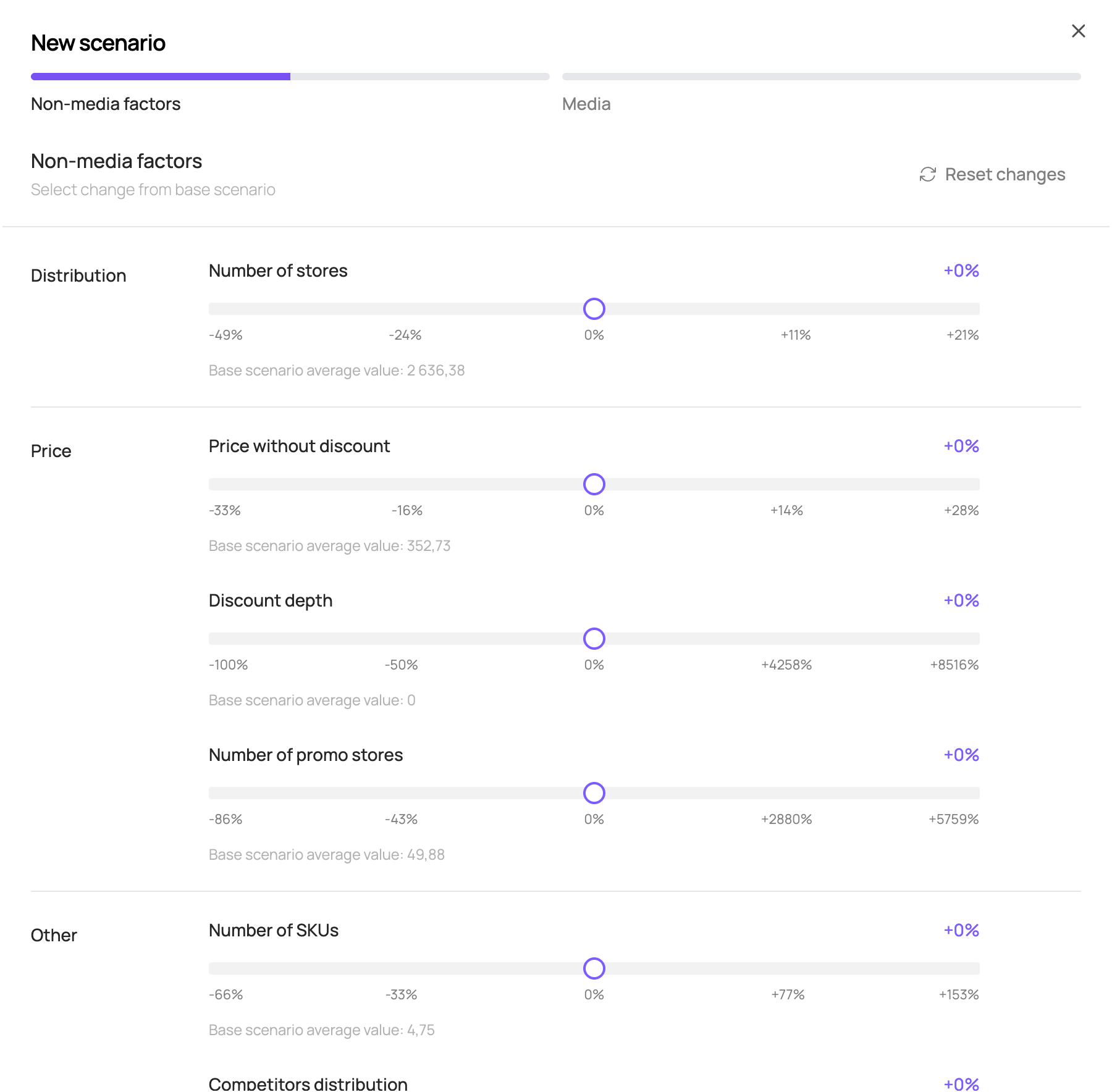
If “Relative to base scenario” was selected, you can increase/decrease each factor relative to the base scenario with sliders. The factor value in each week of the forecast period changes by the same percentage relative to the base scenario.
The slider shows the percentage change of the factor relative to the base value; below the slider you can see the factor's average value in the base scenario and its current value after the change.
The range in which factor values can be changed is calculated for each factor from its change over the historical period and is shown below the slider.
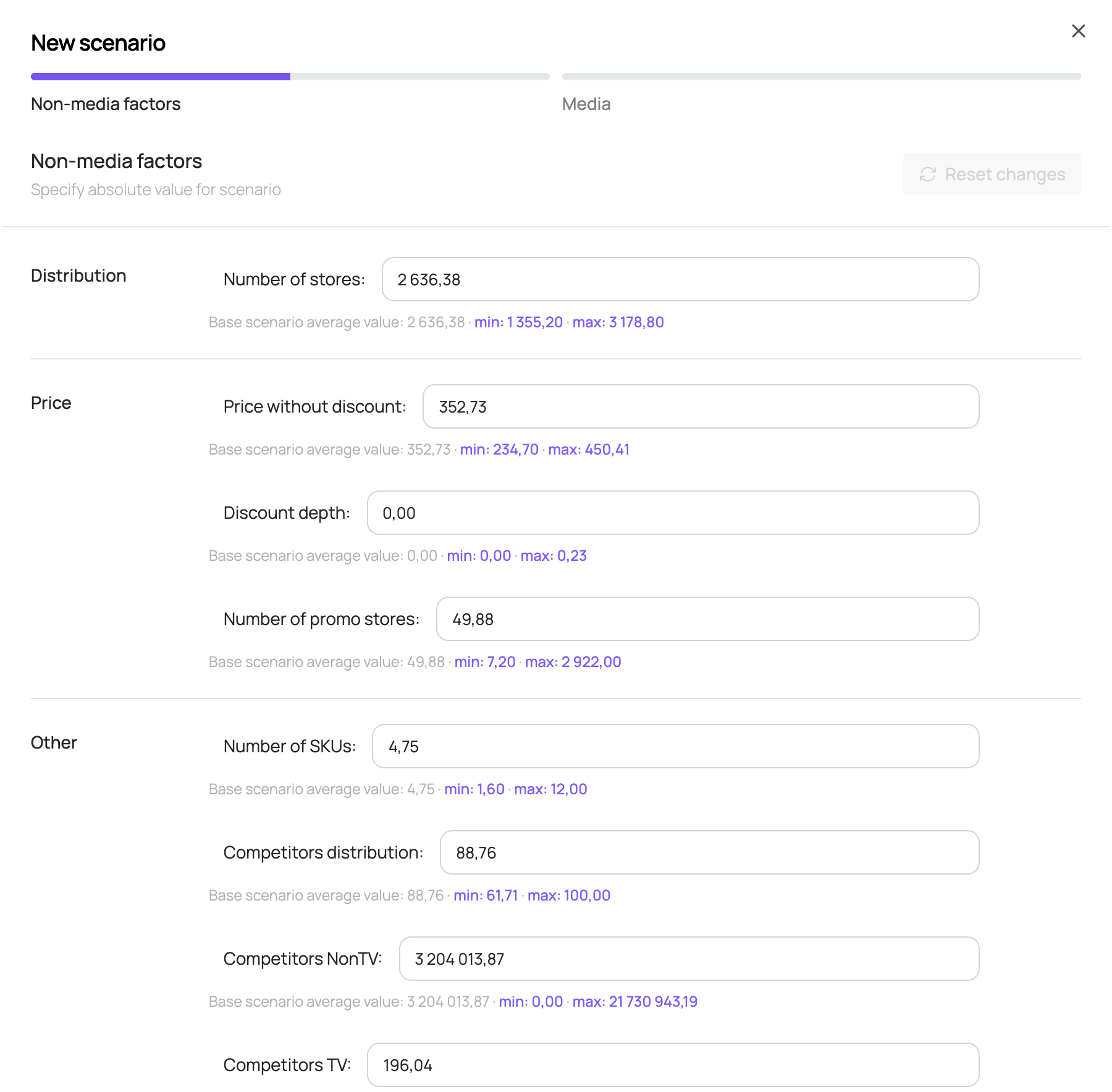
If “Exact value” was selected, set a value for each factor for the forecast period. This value is applied to all weeks of the forecast period.
A factor value can only be entered within the min–max interval shown below the input field for each factor.
Media factors
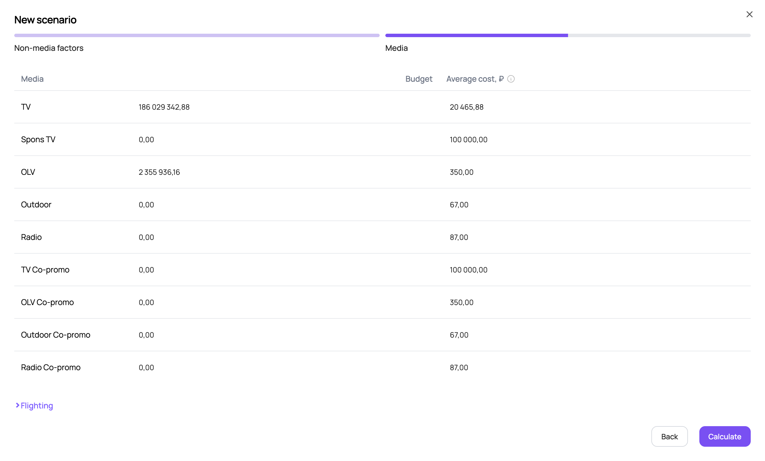
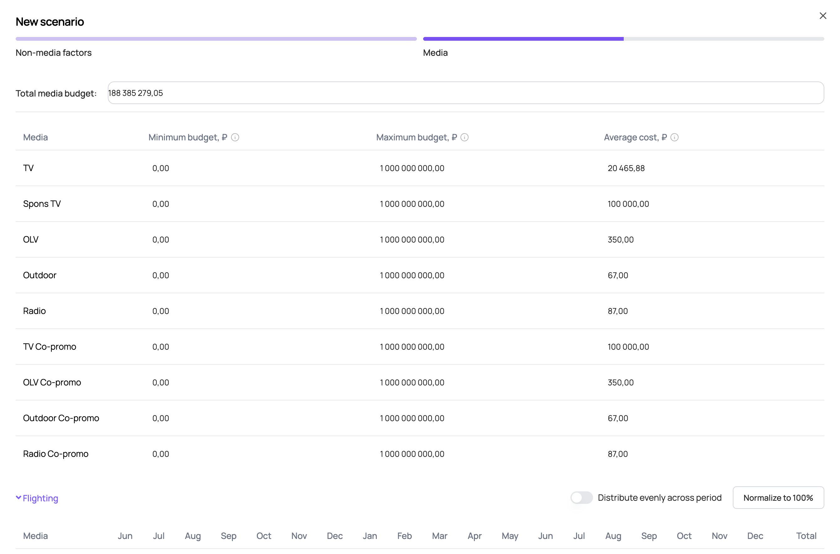
If “Fixed split calculation” was selected, enter the total budget for the forecast period and the cost per placement volume unit for each media channel. The volume units of each media channel used in the model may vary depending on the source data used for modelling. Typically, the volume unit for TV is 1 TRP and for other media channels 1 impression / 1000 impressions.
By default, the table contains the base scenario budgets and costs for the media channels that had placements in the last available year. If there were no placements in the last available year, a zero budget and the average cost over the entire historical period are filled in by default.
The average cost is calculated as:
The budgets entered for each channel are divided by the costs, and the resulting placement volumes are distributed across weeks according to the monthly split in the flighting table. To change the flighting, click “Flighting” below the budget table.
If “Maximize sales within a given budget” was selected, fill in the total media budget for the forecast period and the minimum and maximum budget constraints for each media channel; you can also adjust the cost per placement volume unit. The volume units of each media channel used in the model may vary depending on the source data used for modelling. Typically, the volume unit for TV is 1 TRP and for other media channels 1 impression / 1000 impressions.
By default, the table contains the total base scenario budget and the base scenario costs for the media channels that had placements in the last available year. If there were no placements in the last available year, the average cost over the entire historical period is filled in by default.
After you click “Calculate”, the tool selects the optimal media mix to maximise the sales return on media investment, taking into account the budget constraints and costs of each media channel and the monthly split of placement volumes set in the flighting table. To change the flighting, click “Flighting” below the budget table.
Flighting
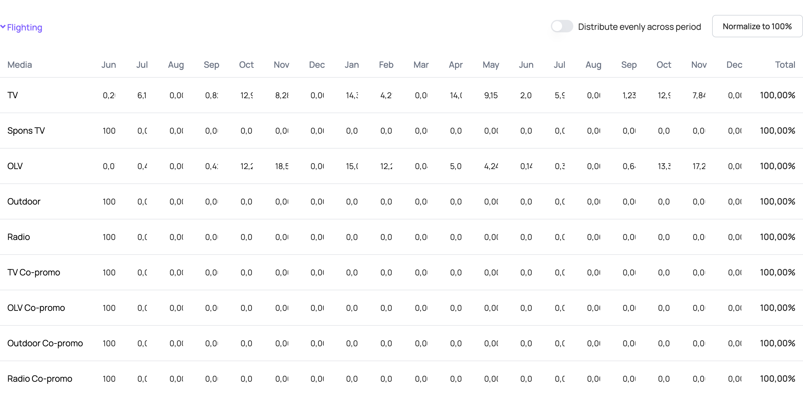
The flighting table shows the share of placement volume for each month of the forecast period. The total for each media channel must be 100%.
By default, the table contains the base scenario flighting for the media channels that had placements in the last available year. Otherwise, 100% is set for the first month of the forecast period.
All values in the flighting table can be changed. For each media channel planned for the forecast period, set the share of placement volume in each month of the forecast period. Within a month, volume is distributed evenly across weeks.
If the total is not 100% after your changes, use “Normalize to 100%” — it proportionally raises/lowers each month's percentage so that the row totals 100%. The “Distribute evenly across period” toggle distributes each media channel's placement volume evenly across all months of the forecast period.
Creating a new scenario — using a template
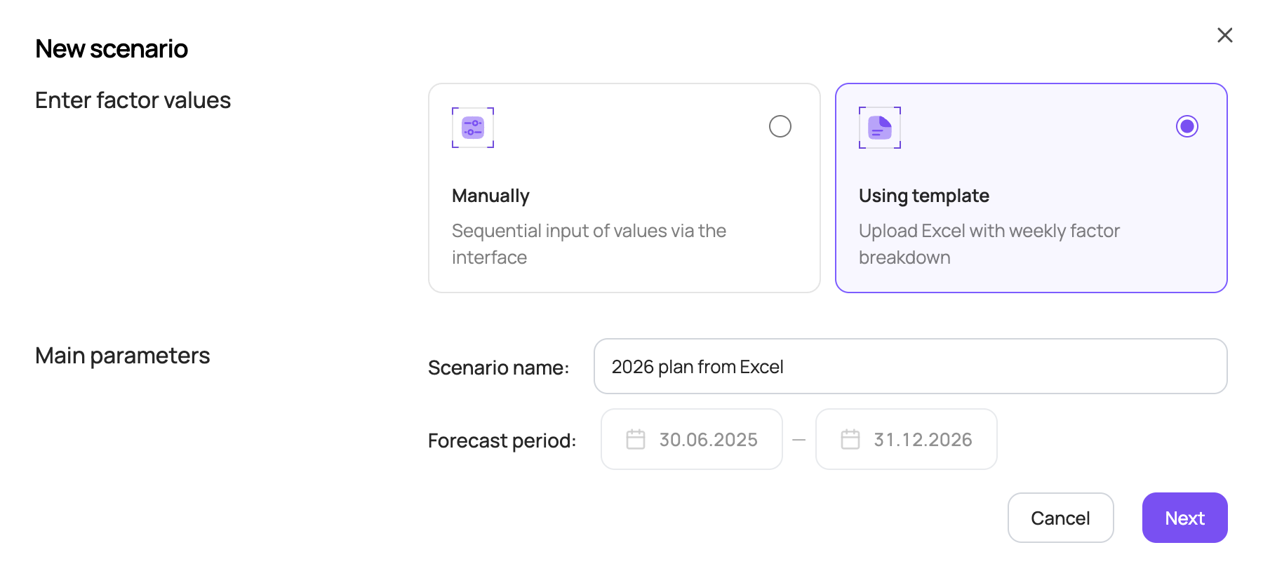
- In the top right corner of the Sales scenarios tab, click “Add scenario”. A new scenario can be created in two ways: manually (via the interface) or using a template (by uploading an Excel file).
- To create a scenario using a template, choose “Using template”, enter the scenario name and click “Next”.
- Download the template to fill in the values of the factors used in the forecast.
The forecast period is shown for reference. To change it, go back to the Sales scenarios page.
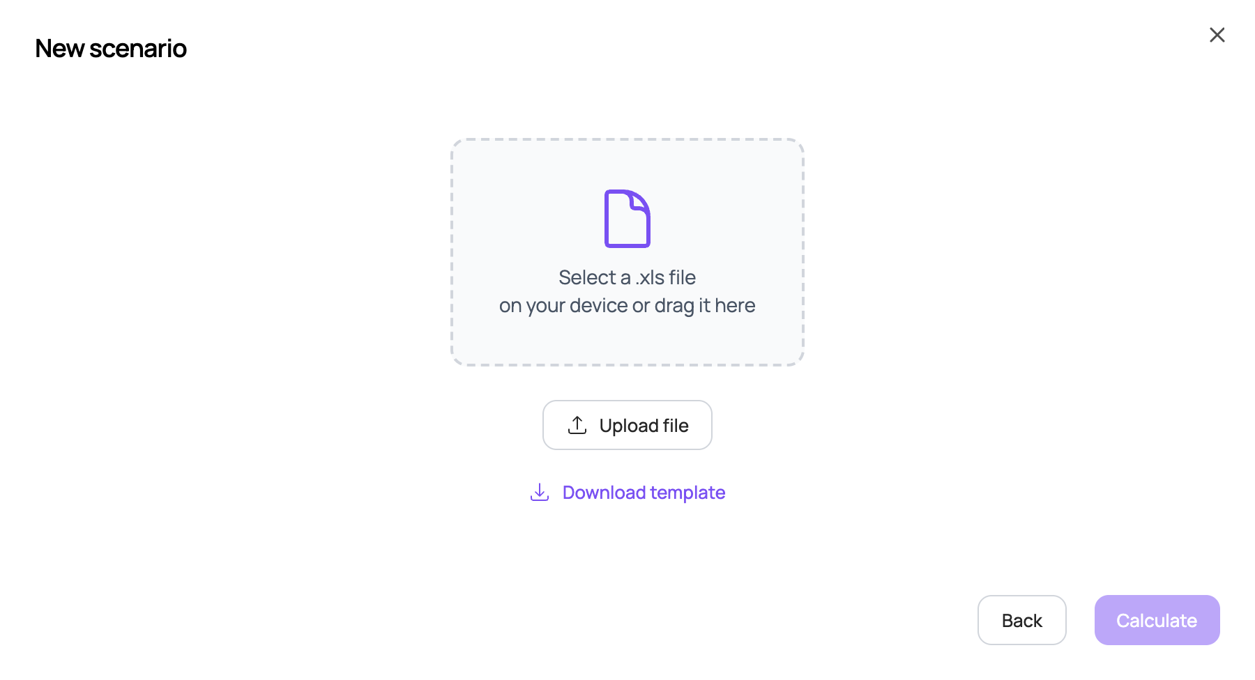
The template is an Excel file with three sheets to fill in. All factor values are entered weekly for the entire period specified in the template.
The template period contains the weeks of the retro period and the forecast period for which there is no actual data included in the model. For example, if the model is built up to mid-2026 and you need to forecast 2027, the template contains the weeks from the second half of 2026 to the end of 2027, which need to be filled in.
| Sheet | What to fill in |
|---|---|
| “Медиа” (Media) sheet | Budgets by media channel. |
| “Стоимость медиа” (Media cost) sheet | The cost per placement volume unit. The volume units of each media channel used in the model may vary depending on the source data used for modelling. Typically, the volume unit for TV is 1 TRP and for other media channels 1 impression / 1000 impressions. |
| “Маркетинг факторы” (Marketing factors) sheet | Values of all other model factors. |
By default, the template is filled in with base values:
- media activity is set to the same budgets and costs as in the same period last year;
- seasonality corresponds to each specific week;
- the category sales factor is forecast by trend;
- other factors use average values over the last 8 available weeks included in the model.
Once the template is filled in, save it, upload it to the scenario and click “Calculate”.
Elasticities
This section lets you build elasticity curves for price and distribution factors, as well as response curves for media channels.
To open the elasticities section, click the button in the menu on the left of the screen; it shows a curve-on-a-chart icon.
At the top of the elasticities section, choose the factor group (price, distribution or media) to build elasticity curves for, as well as the category and brand. Depending on the source data, subcategory, geography and SKU selection may also be available.
Elasticities for price factors
At the top of the “Price” tab, choose the price factor to build elasticity curves for in the “Elasticity factor” field. The set of price factors varies depending on the factors included in the model.

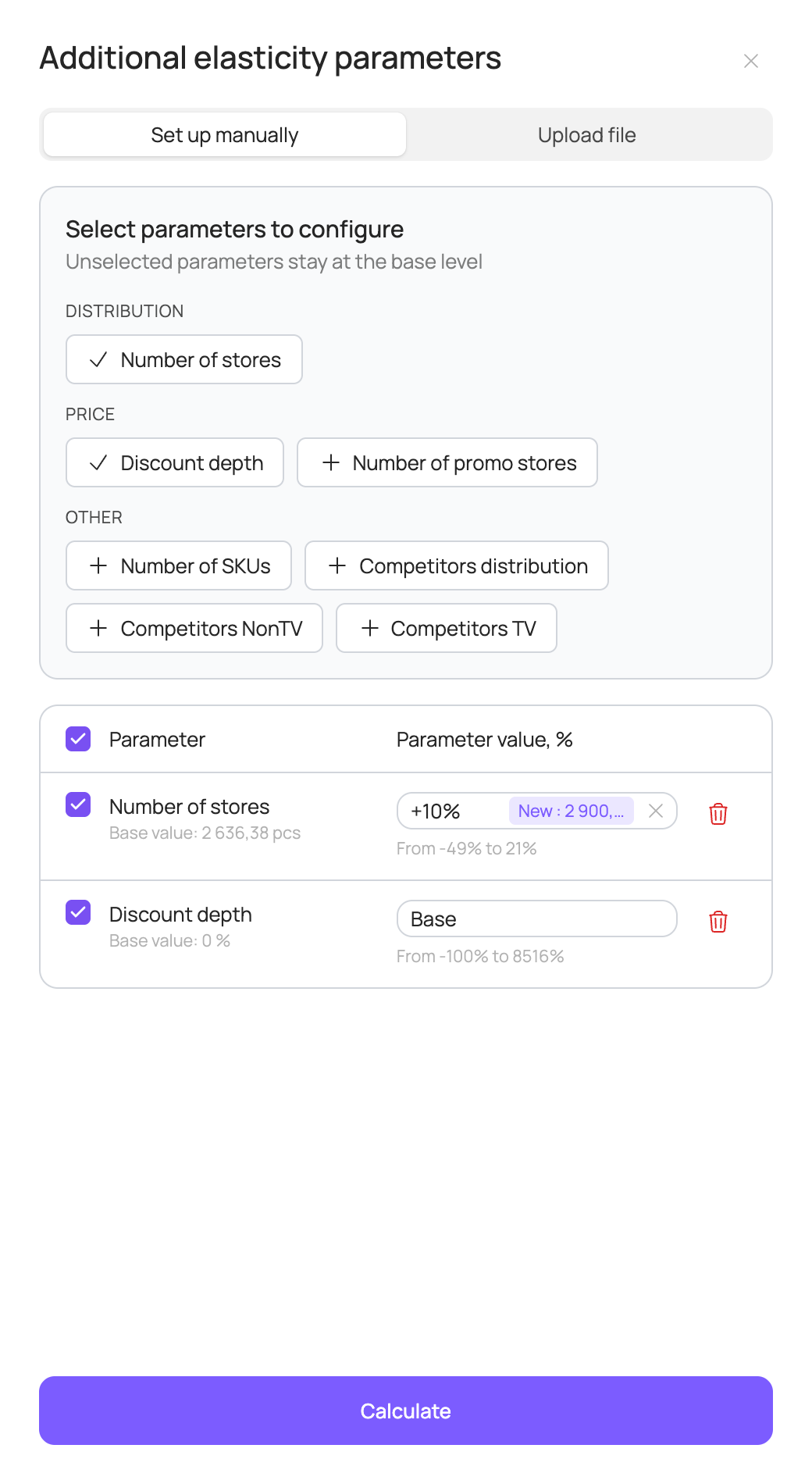
Since all factors in the model are interdependent, the elasticity curve of the selected factor depends on the values of the other factors. To set current or planned values of other factors, click the “Additional parameters” field in the filter panel. The “Additional elasticity parameters” panel offers two modes: “Set up manually” and “Upload file”. The set of factors varies depending on the source data used for modelling.
In “Set up manually” mode, choose the factors you need in the “Select parameters to configure” block and set a percentage change relative to the base value for each of them. Parameters you don't select stay at the base level. Below the input you can see the base and new values of the factor and the allowed range of change.
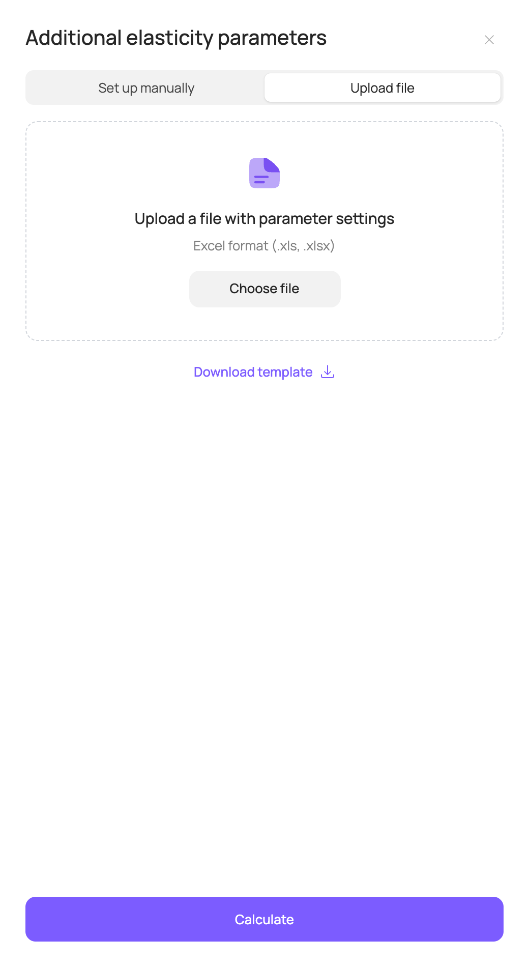
In “Upload file” mode, you can set weekly values of all factors with an Excel file; the elasticity curves use the average weekly values of all factors. To use this option, first download the template (“Download template”), fill it in with your values and then upload it.
By default, factor values are set at the base scenario level. (How base scenario factor values are set is described in the Sales scenarios section.)
Once factor values are set, click “Calculate” at the bottom of the “Additional elasticity parameters” panel or in the centre of the page. If you change parameters after calculation, the “Recalculate curves” button appears.
After calculation, the following 4 charts are shown on the page.
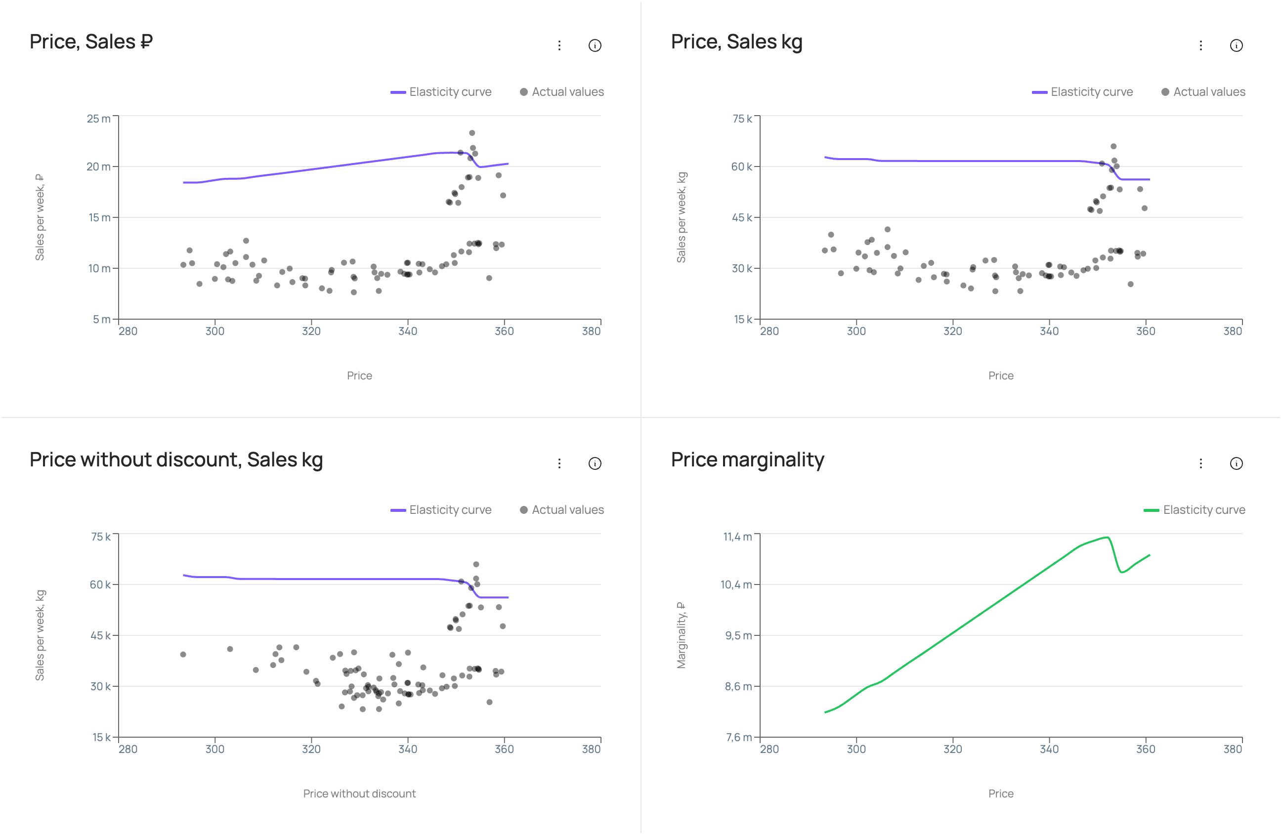
The bottom-left chart shows elasticity for the selected price factor and sales in volume (for example, “Price without discount, Sales kg”). It shows how sales volume depends on the level of the selected price factor: the “Elasticity curve” line is the weekly sales forecast at different values of the price factor with the other factors fixed; the “Actual values” points are actual weekly sales at different values of the price factor, with the other factors not fixed but taking their actual values for each specific week.
The top of the page shows the “Price, Sales ₽” and “Price, Sales kg” charts for price per volume unit and sales in roubles/volume. They show how sales in roubles/volume depend on the price per volume unit: the line is the elasticity curve (weekly sales forecast at different prices per volume unit with the other factors fixed); the points are actual weekly sales at different actual prices per volume unit, with the other factors not fixed but taking their actual values for each specific week.
The bottom-right chart is “Price marginality”. It shows how marginality depends on the price per volume unit.
The unit cost of the product can be entered in the “Unit cost” field in the filter panel.
Elasticities for distribution factors
At the top of the “Distribution” tab, choose the distribution factor to build elasticity curves for in the “Elasticity factor” field. The set of distribution factors varies depending on the factors included in the model.

Values of other factors are set the same way as for price factors: in the “Additional elasticity parameters” panel, manually or with an Excel file. By default, factor values are set at the base scenario level. Once values are set, click “Calculate”.
After calculation, the following 2 charts are shown on the page.
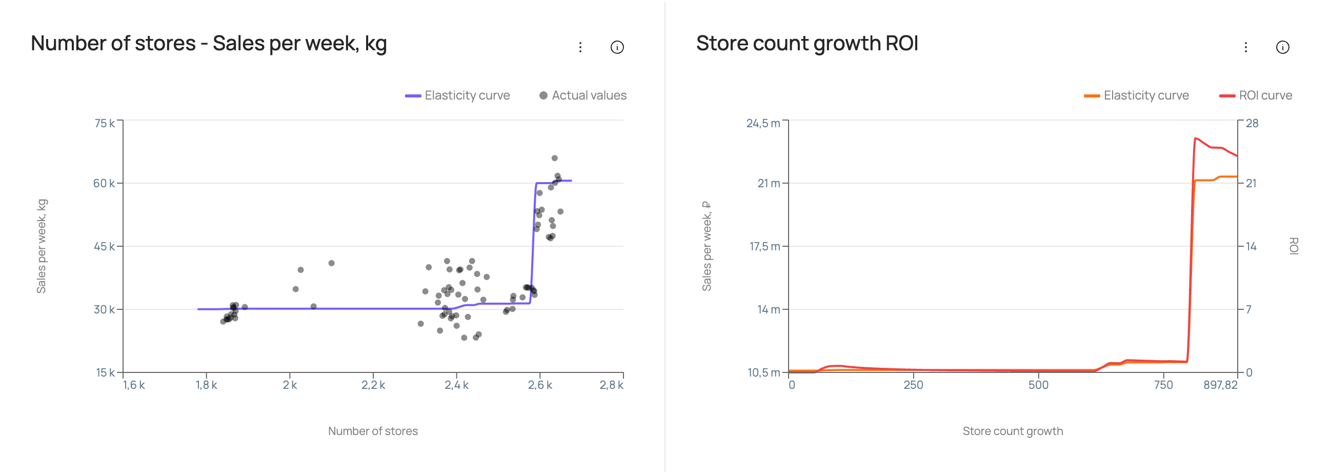
The chart on the left shows how sales volume depends on the values of the selected distribution factor: the “Elasticity curve” line is the weekly sales forecast at different values of the distribution factor with the other factors fixed; the “Actual values” points are actual weekly sales at different actual values of the distribution factor, with the other factors not fixed but taking their actual values for each specific week.
The chart on the right shows the payback of spending on growth of the selected distribution factor. The “Elasticity curve” is the weekly sales forecast in roubles at different levels of growth of the distribution factor relative to its current level (with the other factors fixed). The “ROI curve” is ROI at different levels of growth of the distribution factor relative to its current level (with the other factors fixed).
The cost per unit of distribution factor growth can be entered in the cost field in the filter panel, for example “Cost per store”.
Media response curves
At the top of the “Media” tab, you can change the period for the curves in the “Curves period” field. By default, the year matching the base scenario is selected.
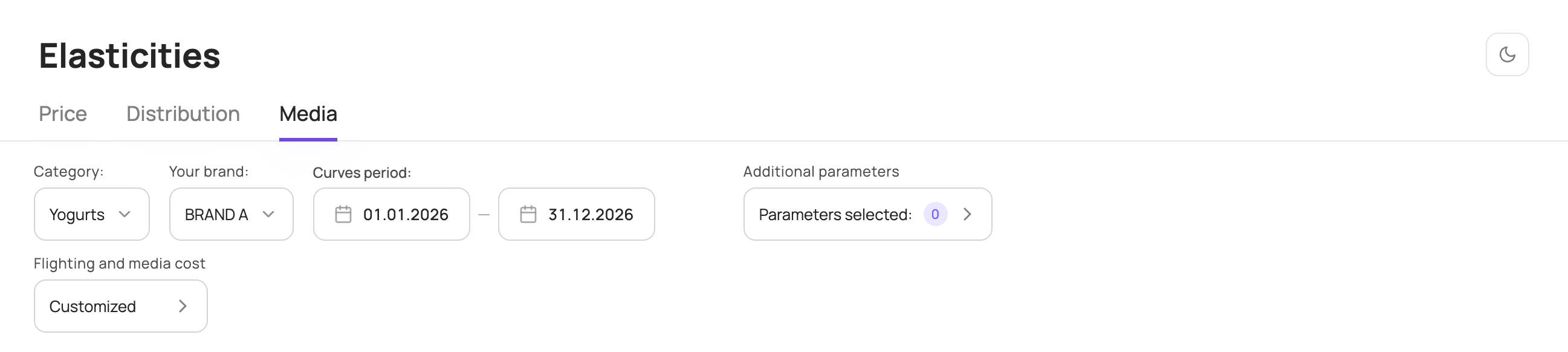
Values of other factors are set in the “Additional elasticity parameters” panel, manually or with an Excel file, as for price factors. The percentage change of a factor is applied to each week of the selected period; in the Excel file you can set factor values for each specific week of the selected period. By default, factor values are set at the base scenario level.
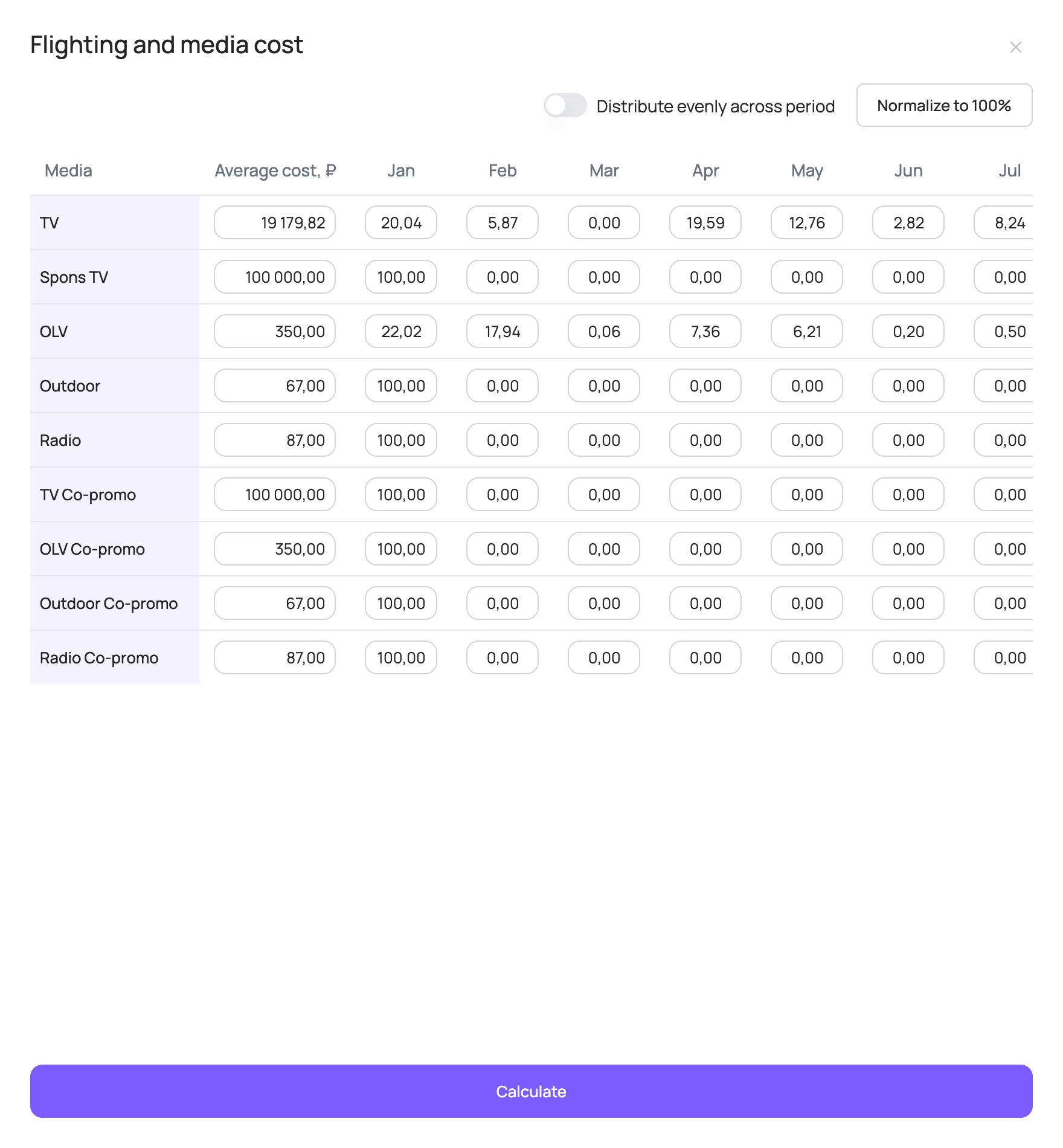
You can also change the flighting and cost settings of media channels. To do this, click the “Flighting and media cost” field in the filter panel. These settings affect the response curve calculation.
For each media channel, the “Average cost, ₽” column shows the cost per volume unit used in the model. The volume units of each media channel used in the model may vary depending on the source data used for modelling. Typically, the volume unit for TV is 1 TRP and for other media channels 1 impression / 1000 impressions.
By default, the table contains the base scenario costs for the media channels that had placements in the last available year. If there were no placements in the last available year, the average cost over the entire historical period is filled in by default.
The average cost is calculated as:
The flighting table shows the share of placement volume for each month of the selected curve period. The total for each media channel must be 100%.
By default, the table contains the base scenario flighting for the media channels that had placements in the last available year. Otherwise, 100% is set for January.
All values in the flighting table can be changed. For each media channel, set the share of placement volume in each month of the selected period. Within a month, volume is distributed evenly across weeks.
If the total is not 100% after your changes, use “Normalize to 100%” — it proportionally raises/lowers each month's percentage so that the row totals 100%. The “Distribute evenly across period” toggle distributes each media channel's placement volume evenly across all months of the period.
Once all cost and flighting settings are set, click “Calculate” at the bottom of the panel: the settings are saved and the response curves are recalculated.
After calculation, the “Media elasticity by budget” chart shows the response curves of media channels for the selected period.
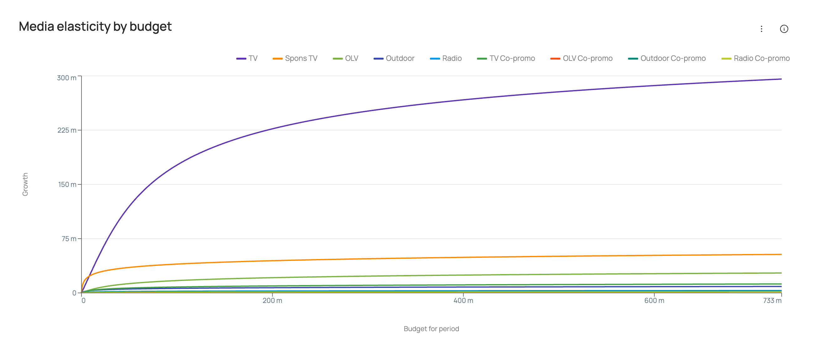
The set of media channels varies depending on the media factors included in the sales models of the category brands.
The chart shows curves of sales growth in roubles against media investment for the selected period. Each point on a curve takes into account the cost per volume unit of the media channel, the distribution of volumes across the selected period and the values of other factors.
Technical charts
This section shows how well the model fits actual data, a detailed decomposition and factor dynamics over the entire historical period, and various model quality metrics.
To open the technical charts, click “Technical Charts” in the top right corner of the main ROI Navigator page.
At the top of the page, choose a category and brand. Depending on the source data used for modelling, subcategory, geography and SKU selection may also be available.

Sales: Actual vs Model
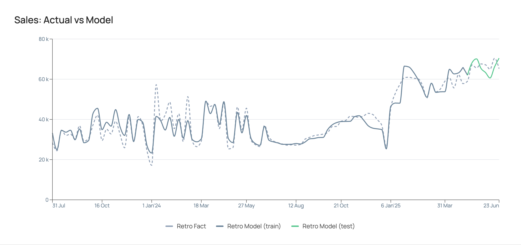
The chart shows weekly dynamics over the entire historical period of actual sales (“Retro Fact”) and modelled sales (“Retro Model”), split into 2 segments: train — the training sample and test — the test sample.
During modelling, all model parameters are fitted on the training sample, and the quality of the resulting model is then assessed on the test sample.
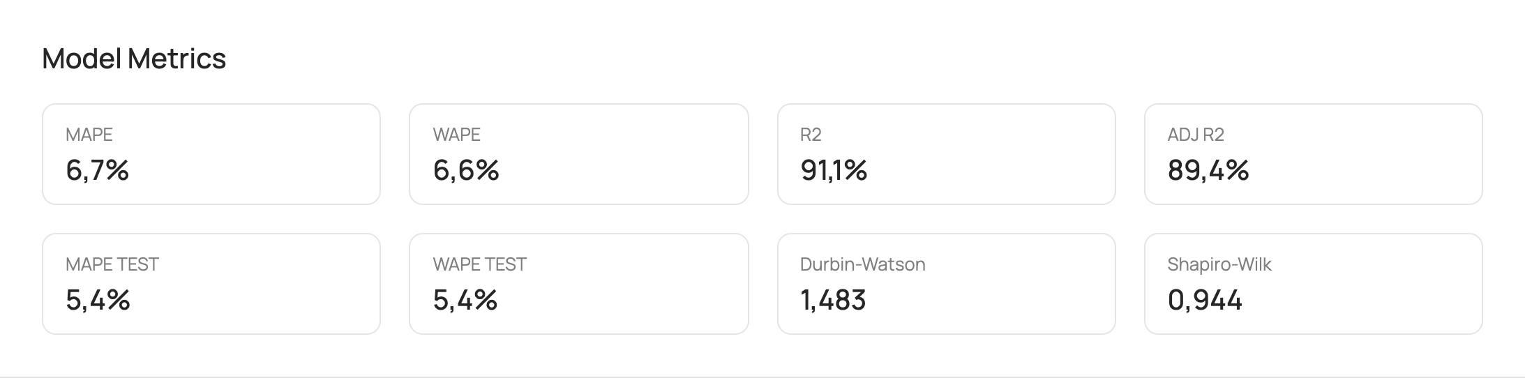
Model Metrics
| Metric | Description |
|---|---|
| MAPE | Mean weekly percentage error of the model; shows by how many percent weekly model sales differ from actual sales on average. Benchmark <15%. |
| WAPE | Weighted percentage error of the model; shows by how many percent total model sales for the entire period differ from actual sales. Benchmark <15%. |
| R2 | Coefficient of determination; shows the share of explained variance, i.e. the percentage of sales fluctuations explained by the model. Benchmark >80%. |
| ADJ R2 | Adjusted coefficient of determination; a modification of the coefficient of determination that accounts for the number of explanatory variables in the model and the sample size. ADJ R2 decreases when irrelevant factors are added and increases only if a new factor actually improves the explanation of the dependent variable's variation. Benchmark >80%. |
| MAPE TEST / WAPE TEST | Percentage errors of the model over the test period, i.e. the last weeks (usually 8) with available actual data. The test period is excluded from the source data when training the model and is used to assess model quality after it is built. Benchmark <15%. |
| Durbin-Watson | Shows whether there is autocorrelation in the model residuals. A DW value between 1.5 and 2.5 indicates no autocorrelation. A DW value between 1 and 1.5 or between 2.5 and 3 indicates weak correlation (below 0.4). |
| Shapiro-Wilk | Tests whether model errors are normally distributed. Values closer to 1 correspond to samples closer to a normal distribution. If p-value ≥ 0.05, the hypothesis of normally distributed residuals is accepted. |
Benchmarks are given for reference: they are not shown in the interface.
Factor Metrics
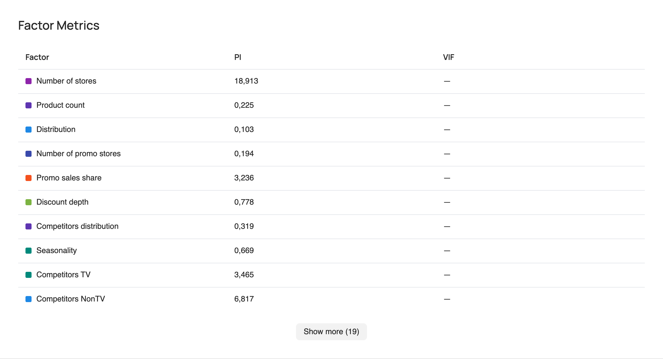
PI — permutation importance shows how much model quality deteriorates if the values of a factor are randomly shuffled. If model quality drops noticeably after shuffling, the factor is considered important; if it barely changes, the factor matters little to the model. The larger the drop in quality, the higher the factor's permutation importance and the more the model relies on it when calculating its contribution to sales.
Decomposition
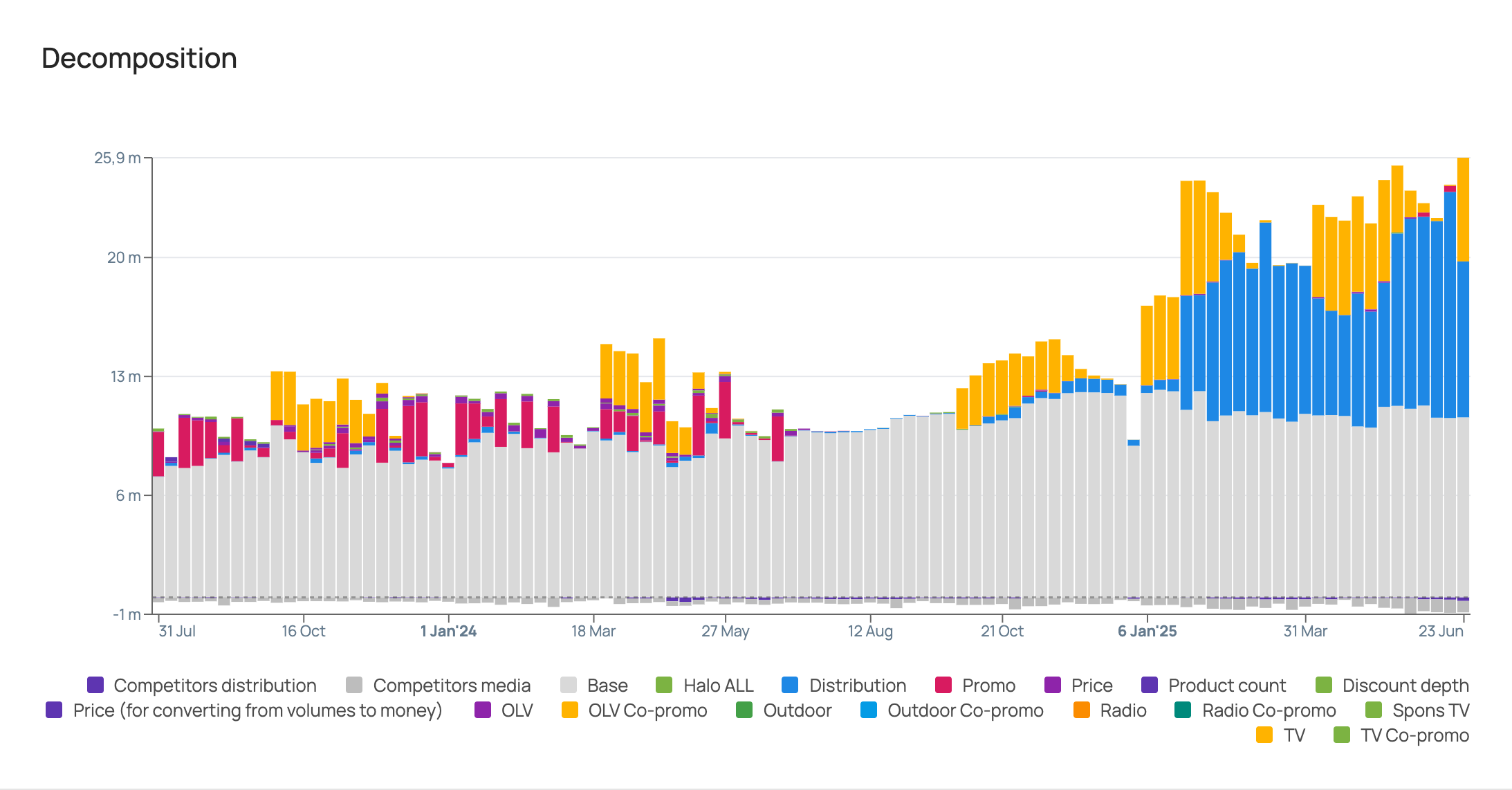
The chart shows the contribution of each factor to brand sales in roubles over the entire historical period.
Factor dynamics
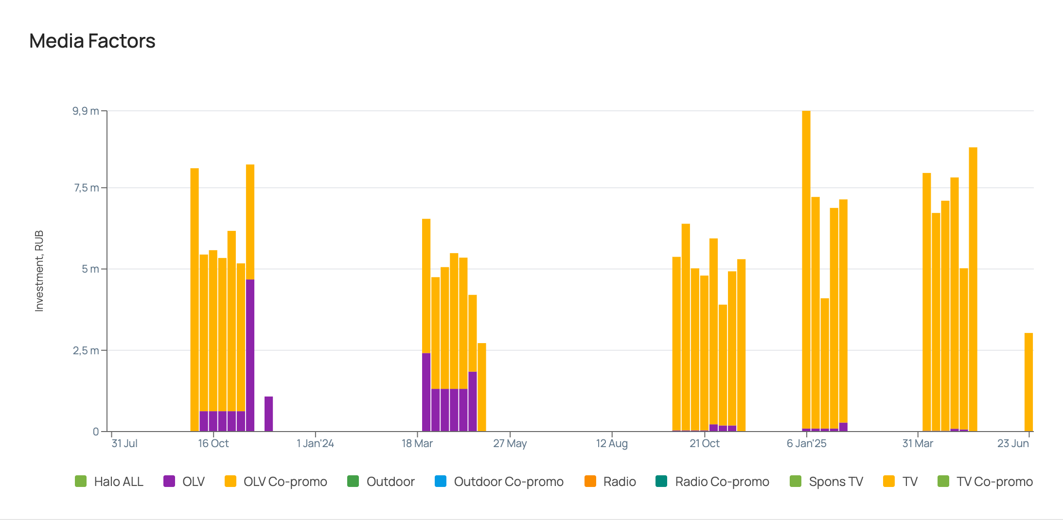
Next come charts with the dynamics of the values of the factors included in the model over the entire historical period.
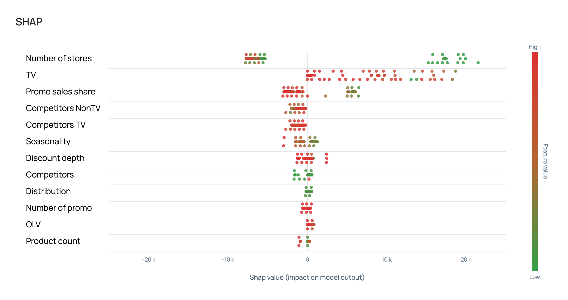
SHAP
The SHAP value of a factor is a numerical estimate of that factor's contribution to the model prediction relative to the average prediction.
A positive SHAP value means the factor increased the prediction; a negative one means it decreased it. The sum of SHAP values across all features plus the base level gives the final model prediction.
The higher the absolute SHAP value, the stronger the factor's influence on the sales forecast.